Lingyan Ou* | Ling Chen
© 2020 IIETA. This article is published by IIETA and is licensed under the CC BY 4.0 license (http://creativecommons.org/licenses/by/4.0/).
OPEN ACCESS
Corporate internet reporting (CIR) has such advantages as the strong timeliness, large amount, and wide coverage of financial information. However, the CIR, like any other online information, faces various risks. With the aid of the increasingly sophisticated artificial intelligence (AI) technology, this paper proposes an improved deep learning algorithm for the prediction of CIR risks, aiming to improve the accuracy of CIR risk prediction. After building a reasonable evaluation index system (EIS) for CIR risks, the data involved in risk rating and the prediction of risk transmission effect (RTE) were subject to structured feature extraction and time series construction. Next, a combinatory CIR risk prediction model was established by combining the autoregressive moving average (ARMA) model with long short-term memory (LSTM). The former is good at depicting linear series, and the latter excels in describing nonlinear series. Experimental results demonstrate the effectiveness of the ARMA-LSTM model. The research findings provide a good reference for applying AI technology in risk prediction of other areas.
deep learning (DL), corporate internet reporting (CIR), risk prediction, long short-term memory (LSTM)
In the Internet era, significant changes have taken place in the way enterprises handle businesses and disclose financial information, owing to the rapid development of information technology (IT). Breaking through the shackles of traditional financial reporting, Corporate internet reporting (CIR) have such advantages as the strong timeliness, large amount, wide coverage, standardized disclosure, high transparency, and openness of financial information [1-4]. The CIR, like any other online information, mainly faces two kinds of risks: the participants on the information transmission chain might suffer losses, and the social factors might exert negative impacts in the disclosure process. Therefore, it is an urgent task to predict the risks of the CIR [5-9].
Currently, CIR risk analysis mainly focuses on the risks in the following areas and their control measures: internal control, commercial secret leakage, CIR diversification, and CIR users [10-14]. Aghaei et al. [15] evaluated the disclosure quality of the CIRs of 600 listed enterprises in the five semi-annual periods between 2018 and 2020, and empirically examined the correlation between disclosure quality and enterprise value; the empirical results prove that the CIR information could effectively reduce the forecast risks of investors. Kumar et al. [16] combines normative research with inductive and deductive approaches to explore the control strategies for CIR disclosure risks, and summarizes the risk control from three aspects: CIR information, CIR tools and CIR security system. By analyzing the synergy and risk transmission path of CIR, Nikoloudis et al. [17] sorted out the relationship between multiple factors affecting risk transmission (e.g. risk source, risk flow, risk carrier, and risk threshold), and provided precautionary suggestions on improving internal control and implementing CIR quality verification.
Based on the cross-platform exchange of financial information, the CIR in eXtensible Business Reporting Language (XBRL) can improve the efficiency of internal information disclosure, while standardizing the financial information of the enterprise. So far, many scholars at home and abroad have investigated XBRL CIRs [18-23]. For instance, Challa et al. [24] constructed a three-dimensional (3D) evaluation index system (EIS) for XBRL CIRs, including the number of mandatory contents, the number of optional contents, and the number of disclosure forms, and empirically analyzed the correlation of CIR information disclosure index with factors like reliability analysis, enterprise size, and capital cost. Zhu et al. [25] highlighted the positive correlations of XBRL CIR with the expected cash flow and enterprise value, and compared the technical features of XBRL against those of Electronic Data Interchange (EDI).
At present, artificial intelligence (AI), which is increasingly sophisticated, has been widely applied in various fields. Considering the sheer size of CIR data, it is meaningful to introduce deep learning (DL) and other AI techniques to risk factor analysis, and risk value calculation, shedding new light on CIR risk prediction. To improve the prediction accuracy of CIR risks of listed enterprises, this paper sets up an CIR risk prediction model based on an improved DL algorithm. After building a reasonable CIR risk EIS, the data involved risk rating and the prediction of risk transmission effect (RTE) were subject to structured feature extraction and time series construction. Based on DL algorithm, autoregressive moving average (ARMA) model was combined with long short-term memory (LSTM) into a combinatory prediction model. The effectiveness of the ARMA-LSTM model was verified through experimental analysis.
Before applying DL algorithms in CIR risk prediction, it is necessary to collect the data related to the risk evaluation indices. For CIR risks, the evaluation indices need to reflect all the features of the relevant data of the CIR. Under the premise of comparability and continuity, this paper makes full use of all financial information resources of the target enterprises (e.g. financial statements, income statements, and balance sheets) to select the evaluation indices, and minimizes the impact of a single index on the entire EIS.
Because DL algorithms can analyze complex functions, a total of five indices, including media structural risk, CIR technical risk, opportunistic risk, internal management risk, and monitoring risk, were taken as the primary indices for CIR risk prediction. The five primary indices are supported by 30 secondary indices. Our three-layer EIS is detailed as follows:
Layer 1 (Goal):
R={CIR risk}.
Layer 2 (Primary indices)
R={R1, R2, R3, R4, R5}={Media structural risk, CIR technical risk, Opportunistic risk, Internal management risk, Monitoring risk}
Layer 3 (Secondary indices)
R1={R11, R12, R13, R14, R15}={Media technology risk, Media information risk, Media knowledge risk, Media public opinion risk, Media political risk}.
R2={R21, R22, R23, R24}={Financial information storage risk, Accounting data operation risk, Accounting processing and query risk, Computer virus prevention measures}.
R3={R31, R32, R33, R34, R35, R36}={Opportunistic risk during preparation, Opportunistic risk during accounting information generation, Opportunistic risk during compilation, Opportunistic risk during verification and review, Opportunistic risk during information transmissions, Opportunistic risk during information disclosure}.
R4={R41, R42, R33, R34}={Funding management risk, Investment management risk, Operation fund risk, Profit distribution risk}.
R5={R51, R52, R53, R54, R55}={Budget management risk, Accounting control risk, Quota control risk, Expense control risk, Investment monitoring risk}.
Considering the high number of indices being selected and the fact that some index data are missing or difficult to obtain, the missing items or abnormal items should be deleted, depending on the enterprises to be evaluated. In addition, the various indices must be normalized to ensure the quality of evaluation. Otherwise, the prediction effect will be undesirable, because of the lag of unstructured data (e.g. the interpretations of the CIR by relevant analysts) and the diversity of the CIRs in disclosure rule and risk source. Therefore, this paper extracts feature factors from CIR risk evaluation indices, analyzes the extracted feature factors under the CIR single-factor test framework, and thereby builds up a multi-factor feature library for CIR risk prediction.
This paper mainly carries out structured feature extraction from the data on CIR risk evaluation indices involved in risk rating and RTE prediction. As shown in Figure 1, the extraction of feature factors consists of two steps: structured feature extraction, and time series construction.
Figure 1. The extraction of feature factors
3.1 Feature factors of risk rating
Risk rating is to analyze the basic financial situation disclosed by the CIR, and derive the risk level of the enterprise, according to the CIR risk formation mechanism and the established EIS. In traditional risk rating, the terms and measuring conditions vary with the third-party risk assessment agencies.
With reference to other research reports and statistics, this paper divides CIR risks into five levels, namely, level A (strongly significant risk), level B (significant risk), level C (general risk), level D (insignificant risk), and level E (strongly insignificant risk), which respectively correspond to the five ranges of the quantitative values of CIR risks. For each CIR, the contents to be measured were extracted through regular matching and pattern matching. Then, the CIR risk was quantified according to all the contents of the evaluation indices. Figure 2 presents an example on the quantitative values of CIR risk levels.
Figure 2. The quantitative values of CIR risk levels
(1) Risk rating consistency factor
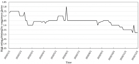
Since the release time of CIR is relatively fixed, the quantitative values of CIR risk levels can serve as the time series feature factors in CIR risk prediction. But the evaluation indices are generally collected in different periods. It is necessary to convert the discrete data for risk rating into a time series.
Figure 3. The risk rating of index R21 obtained by the consistency factor
The risk rating consistency factor was introduced for a single evaluation index. The factor counts the factor values of the index in the current period corresponding to all the historical CIRs of the enterprise. In this way, full consideration is given to the consistent risk rating of the index in the historical financial information of the enterprise.
Let R={r1, r2, r3, …, rn} be the CIRs released for an index between time t-n to time t, where ri is the risk rating of the i-th CIR on that index in period [t-n, t]. Then, the consistency factor St of that index at time t can be calculated as the weighted sum of all risk ratings:
${{S}_{t}}=\sum\limits_{i=t-n}^{t}{\left( {{\omega }_{i}}\cdot \frac{\sum\limits_{i=t-n}^{t}{\left( {{\lambda }_{i}}\cdot \eta _{1}^{t-i} \right)}}{Sum({{r}_{i}})} \right)}$ (1)
where, ωi is the weight of the i-th CIR; η1 is the attenuation factor; λi is the quantitative value of the CIR risk level corresponding to the index in ri. Figure 3 provides the risk rating of index R21 obtained by the consistency factor.
(2) Risk rating change factor
Based on the consistency factor, the risk rating change factor further considers the deviation of the predicted CIR risk from the actual value, which is induced by the interaction and mutual influence between various uncertain factors throughout information transmission. By the exponential weighted average method, the risk rating change factor was characterized as the difference between the risk ratings of the current period and the previous period, which are obtained by the consistency factor, processed by time smoothing and weighting:
${{M}_{t}}={{\eta }_{2}}{{S}_{t}}+(1-{{\eta }_{2}}){{M}_{t-1}}$ (2)
where, St is the consistency factor at time t; Mt−1 is the change factor of the risk rating of the previous period; η2 is the time attenuation factor.
(3) Risk rating adjustment factor
The risk rating adjustment factor was designed based on the quantitative values of CIR risk rating, after limiting the selection of evaluation indices for principal components and the time periods. This factor could accurately reflect how the quantitative values of risk rating vary with the key evaluation indices.
The risk rating adjustment factor Qt was determined by counting the adjustment events qi of key evaluation indices. The release time of new CIR was taken as the reference time for the occurrence of adjustment event. Then, the adjustment events were divided into core and non-core events. The core events refer to the adjustment of a general index into a key index, that is, the increase of the consistency factor; the non-core events have the opposite meaning.
During the statistical process, each core adjustment event was given +1 point, while each non-core event was given -1 point. Then, the adjustment factor can be defined as the time attenuated weighted sum of the scores of all adjustment events of the index between time t-n and time t:
${{Q}_{t}}=\sum\limits_{i=t-n}^{t}{\eta _{3}^{i}}\cdot \sum\limits_{j=1}^{m}{{{v}_{j}}}$ (3)
where, η3 is the time attenuation factor; vj is the score of the j-th adjustment event between time t-n and time t.
3.2 Feature factors of RTE
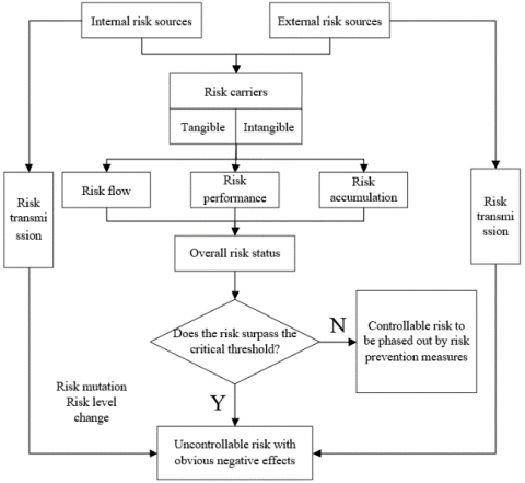
The risk rating is an important way to identify the focus of CIR risk control. Apart from that, it is of even greater importance to predict the interaction between the risk transmission factors of CIR risks. Figure 4 illustrates the correlations between the risk transmission factors of CIR risks. These correlations need to be quantified accurately by analyzing the situation of the risk transmission factors, in the light of the relevant data on the risk evaluation indices.
Figure 4. The correlations between the risk transmission factors of CIR risks
(1) RTE prediction consistency factor
Similar to the risk rating consistency factor, the discrete RTE values between two risk carriers should be converted into a time series through a suitable quantification method. The calculation of RTE prediction consistency factor is time sensitive. With the elapse of time, the RTE of the same path will gradually change. As a result, the RTE prediction consistency factor was not calculated based on specific time points. Instead, the factor was divided into the prediction value u1 at time b, the prediction value u2 at time b+Δb, and the prediction value u3 at time b+2Δb, with Δb being the width of time window. The specific values of u1, u2, and u3 will vary in the CIR disclosure process. The RTE prediction consistency factor can be calculated by:
${{S}_{ut}}=\sum\limits_{i=t-n}^{t}{\left( {{\omega }_{i}}\cdot \frac{\sum\limits_{i=t-n}^{t}{\left( {{\mu }_{i-u}}\cdot \eta _{4}^{t-i} \right)}}{Sum({{r}_{i-u}})} \right)}$ (4)
$S_{u B}=\left\{\begin{array}{lr}S_{u b} & k=0 \\ S_{u\left(b_{u}+\Delta b\right)} & k=1 \\ S_{u\left(b_{u}+2 \Delta b\right)} & k=2\end{array}\right.$ (5)
where, Sut is the predicted value of the RTE prediction consistency factor between time t-n and time t; ri-u is the predicted value of the RTE in the i-th part of the CIR; μi-u is the quantitative value of the predicted RTE corresponding to the CIR in ri-u; η4 is the time attenuation factor; SuB is the predicted value of the RTE prediction consistency factor under the time window with the width of Δb; k is the number of time windows.
(2) RTE prediction change factor
Similar to the risk rating change factor, the RTE prediction change factor further considers the deviation of the predicted RTE from the actual value, which is induced by the interaction and mutual influence between various risk carriers along with the moving time window. Because it involves time series state conversion, the RTE prediction change factor needs to be calculated referring to the computing strategy for the RTE prediction consistency factor:
${{M}_{ut}}={{\eta }_{5}}{{S}_{ut}}+(1-{{\eta }_{5}}){{M}_{u}}_{(t-1)}$ (6)
$M_{u B}=\left\{\begin{array}{ll}M_{u b} \quad k=1 \\ M_{u\left(b_{u}+\Delta b\right)} & k=2 \\ M_{u\left(b_{u}+2 \Delta b\right)} & k=3\end{array}\right.$ (7)
where, Mut is the RTE prediction change factor between time t-n and time t; Sut is the RTE prediction consistency factor at time t; Mt−1 is the RTE prediction change factor in the previous period; η5 is the time attenuation factor.
The ARMA is a time series analysis model, which couples the autoregressive (AR) model with the moving average (MA) model. The i-th order AR model can be expressed as:
$AR(i)=\left\{ \begin{align} & {{c}_{t}}={{\alpha }_{0}}+{{\alpha }_{1}}{{c}_{t-1}}+{{\alpha }_{2}}{{c}_{t-2}}+\cdots +{{\alpha }_{i}}{{c}_{t-i}}+{{\tau }_{t}},{{\alpha }_{i}}\ne 0 \\ & W\left( {{\tau }_{t}} \right)=0,Var\left( {{\tau }_{t}} \right)={{\sigma }_{s}}^{2},W\left( {{\tau }_{t}}{{\tau }_{v}} \right)=0,v\ne t \\ & \text{ }W\left( {{\tau }_{t}}{{\tau }_{v}} \right)=0,\forall v<t \\\end{align} \right.\text{ }$ (8)
when α0=0, AR(i) becomes a centralized AR model. The j-th order MA model can be expressed as:
$MA(j)=\left\{ \begin{align} & {{c}_{t}}=\varphi +{{\tau }_{t}}-{{\beta }_{1}}{{\tau }_{t-1}}-{{\beta }_{2}}{{\tau }_{t-2}}-\cdots -{{\beta }_{j}}{{\tau }_{t-j}},{{\beta }_{j}}\ne 0 \\ & W\left( {{\tau }_{t}} \right)=0,Var\left( {{\tau }_{t}} \right)={{\sigma }_{s}}^{2},W\left( {{\tau }_{t}}{{\tau }_{v}} \right)=0,v\ne t \\ & \text{ }W\left( {{\tau }_{t}}{{\tau }_{v}} \right)=0,\forall v<t \\\end{align} \right.\text{ }$ (9)
when ϕ=0, MA(i) becomes a centralized MA model. Then, the ARMA model can be expressed as:
$ARMA(i,j)=\left\{ \begin{align} & {{c}_{t}}={{\alpha }_{0}}+{{\alpha }_{1}}{{c}_{t-1}}+\cdots +{{\alpha }_{i}}{{c}_{t-i}} \\ & +{{\tau }_{t}}-{{\beta }_{1}}{{\tau }_{t-1}}-{{\beta }_{2}}{{\tau }_{t-2}}-\cdots -{{\beta }_{j}}{{\tau }_{t-j}} \\ & \text{ }{{\alpha }_{i}}\ne 0{{\beta }_{j}}\ne 0\text{ } \\ & W\left( {{\tau }_{t}} \right)=0,Var\left( {{\tau }_{t}} \right)={{\sigma }_{s}}^{2},W\left( {{\tau }_{t}}{{\tau }_{v}} \right)=0,v\ne t \\ & \text{ }W\left( {{\tau }_{t}}{{\tau }_{v}} \right)=0,\forall v<t \\\end{align} \right.$ (10)
when α0=0, ARMA(i, j) becomes a centralized ARMA model.
Three steps are necessary to build an ARMA model for CIR risk prediction: order identification (solving the sum through correlation analysis), parameter estimation (predicting model parameters by Gaussian maximum likelihood estimation), and data prediction (verifying the effectiveness of the model by the Akaike information criterion (AIC), and outputting the risk rating and RTE prediction).
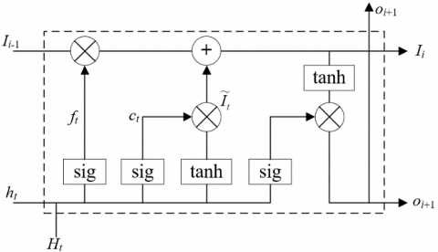
Figure 5 presents the structure of a neuron in the deep neural network (DNN) of LSTM. Different from other neural networks (NN), the neurons of the LSTM operate like a conveyor belt. Except for a few linear interactions, it is easy to keep all the other information flowing between the neurons.
Figure 5. The structure of a neuron in LSTM
To remove or add information to the neuron state, the LSTM have three gating units in each neuro, namely input gate, forget gate, and output gate. The gates selectively control the passage of information, using sigmoid function and multiplication operation.
The forget gate reads the risk rating and RTE perdition ht-1 of the previous moment and the input of the current moment Ht, and outputs a number in [0, 1] for the state of each neuron. The closer the number is to 1, the greater the probability of discarding the information; the closer the number is to 0, the greater the probability of retaining the information:
${{f}_{t}}=Sigmoid([{{h}_{t-1}},{{H}_{t}}]\cdot {{W}_{f}}+{{\varepsilon }_{f}})$ (11)
The input gate determines which new information should be stored in the neuron state. The sigmoid function is used to determine the updated information, while the tanh function is called to create a vector of the new candidate value to be added to the neuron state:
${{c}_{t}}=sigmoid([{{h}_{t-1}},{{H}_{t}}]\cdot {{W}_{c}}+{{\varepsilon }_{c}})\text{ }$ (12)
$\widetilde{I}_{t}=\tanh \left(W_{\tilde{I}} \cdot\left[O_{t-1}, I_{t}\right]+\varepsilon_{\tilde{I}}\right)$ (13)
Then, the old neuron state will be updated. To discard some information, the new candidate value can be calculated by:
${{I}_{t}}={{I}_{t-1}}\cdot f{}_{t}+{{c}_{t}}\cdot {{\tilde{I}}_{t}}$ (14)
The output gate relies on sigmoid function to determine which information should be outputted. Then, the tanh function is called to obtain a value in [-1, 1]. The value will be multiplied with the output of sigmoid, forming to final output:
${{o}_{i+1}}=\alpha +\beta \cdot {{y}_{t}}\tanh \left[ {{I}_{t}} \right]\text{ }$ (15)
${{y}_{t}}=sigmoid([{{h}_{t-1}},{{H}_{t}}]\cdot {{W}_{y}}+{{\varepsilon }_{y}})$ (16)
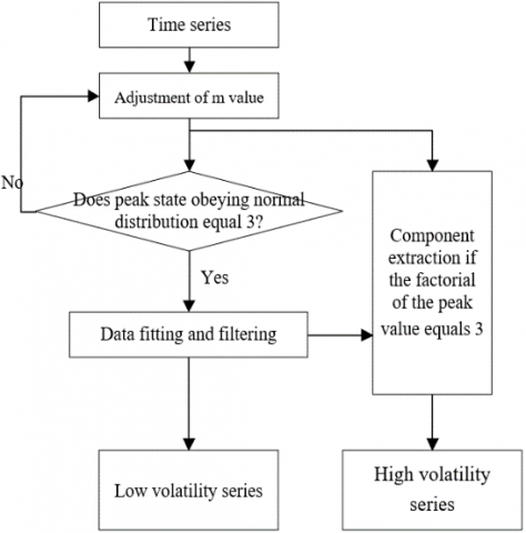
In practical applications, risk ratings and RTE predictions are often converted into time series. But the high volatility of time series cannot be effectively described by ARMA or LSTM alone.
To solve the problem, the risk ratings and RTE predictions were converted into the corresponding time series {Pt}. Then, the time series was decomposed into a high volatility series and a low volatility series by the filtering algorithm in Figure 6:
${{P}_{t}}=LO{{W}_{t}}+HIG{{H}_{t}}\text{ }$ (17)
Figure 6. The workflow of time series decomposition
To obtain better prediction effect, the low volatility series was predicted by AMAR model, and the high volatility series was predicted by LSTM model. The former is good at depicting linear series, and the latter excels in describing nonlinear series. The ARMA model can be defined as:
$LO{{W}_{t}}=ARMA\left( {{L}_{t-1}},{{L}_{t-2}},\cdots ,{{L}_{t-i}},{{\tau }_{t}},{{\tau }_{t-1}},\cdots ,{{\tau }_{t-j}} \right)\text{ }$ (18)
The linear function can be expressed as:
$\left\{ \begin{align} & LO{{W}_{t}}={{\alpha }_{0}}+{{\alpha }_{1}}{{L}_{t-1}}+\cdots +{{\alpha }_{i}}{{L}_{t-i}} \\ & +{{\tau }_{t}}-{{\beta }_{1}}{{\tau }_{t-1}}-{{\beta }_{2}}{{\tau }_{t-2}}-\cdots -{{\beta }_{j}}{{\tau }_{t-j}} \\ & \text{ }{{\alpha }_{i}}\ne 0,{{\beta }_{j}}\ne 0\text{ } \\ & W\left( {{\tau }_{t}} \right)=0,Var\left( {{\tau }_{t}} \right)={{\sigma }_{s}}^{2},W\left( {{\tau }_{t}}{{\tau }_{v}} \right)=0,v\ne t \\ & \text{ }W\left( {{\tau }_{t}}{{\tau }_{v}} \right)=0,\forall v<t \\\end{align} \right.$ (19)
For the high volatility series, the risk rating was predicted by three steps forward based on the time window obtained by formulas (5) and (6):
$HIG{{H}_{t}}=LSTM\left( {{S}_{t-1}},{{S}_{t-2}},\cdots ,{{S}_{t-N}} \right)+{{\theta }_{t}}$ (20)
To predict the RTE, the time series St in the above formula was replaced with time series Sut, and the value of time series {Pt} was predicted by formulas (18) and (9), using the time window obtained from formula (6).
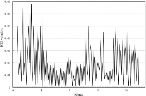
The CIR risk prediction experiments were carried out on the information disclosed by the CIR of a listed enterprise in 2019. Figure 7 shows the experimental results of structured feature extraction based on the original time series. Subgraphs (a) and (b) are the volatility curves of risk ratings and RTE predictions, respectively. It can be seen that the traditional time series prediction model ARMA did not achieve ideal prediction effect, despite its excellence in solving traditional time series problems. This is because the model is constructed based on statistical principles, and the CIR is affected by various risk factors.
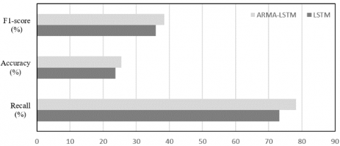
Figure 8 compares the risk prediction results of LSTM and those of ARMA-LSTM. The prediction quality was evaluated by F1-score, accuracy, and recall. The accuracy and recall refer to the proportion of strongly risky data in the data series and that of positive samples in the strongly risky data, respectively. It can be seen that the ARMA-LSTM clearly outperformed the LSTM in all three metrics.
(a)
(b)
Figure 7. The volatility of feature factors
Figure 8. The effects of ARMA on risk prediction
(a) LSTM
(b) ARMA-LSTM
(c) LSTM
(d) ARMA-LSTM
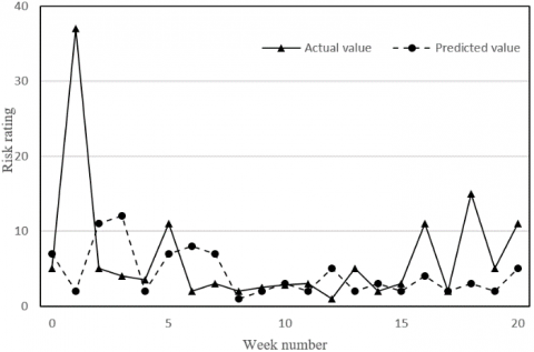
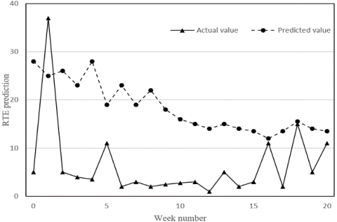
Figure 9. The effects of ARMA on feature factor predictions
Figure 9 compares the feature factor predictions of LSTM and those of ARMA-LSTM. The risk ratings and RTE predictions are contrasted with the actual values in the four subgraphs. The results in Figure 9 further confirm the above conclusions.
Table 1. The risk predictions with time windows of different widths
|
Predictions |
LSTM |
Width of time window |
|||
|
1 week |
2 weeks |
3 weeks |
4 weeks |
||
|
F1-score (%) |
36.87 |
35.64 |
35.76 |
35.77 |
|
|
Accuracy (%) |
30.23 |
27.47 |
27.01 |
29.94 |
|
|
Recall (%) |
78.23 |
75.14 |
72.48 |
75.87 |
|
|
ARMA-LSTM |
Width of time window |
||||
|
1 week |
2 weeks |
3 weeks |
4 weeks |
||
|
F1-score (%) |
46.44 |
45.48 |
44.55 |
43.47 |
|
|
Accuracy (%) |
34.61 |
32.49 |
33.57 |
33.96 |
|
|
Recall (%) |
80.42 |
81.49 |
81.56 |
82.21 |
|
Table 2. The CIR risk predictions of different models
|
Method |
Prediction effects |
||
|
F1-score (%) |
Accuracy (%) |
Recall (%) |
|
|
SVM |
34.69 |
27.63 |
76.85 |
|
BPNN |
36.57 |
28.71 |
76.94 |
|
DNN |
38.15 |
29.47 |
77.48 |
|
LSTM |
37.98 |
28.45 |
76.36 |
|
ARMA-LSTM |
44.76 |
33.42 |
81.35 |
Table 1 compares the risk predictions of LSTM and those of ARMA-LSTM with time windows of different widths. Obviously, the recall reached the highest level, when the time window is 1 week in width. The reason is that taking a week as the cycle can simultaneously optimize the quality and computing load of CIR risk prediction. Hence, the risk prediction effect of the LSTM with a week as the time scale achieved better results.
Furthermore, the proposed ARMA-LSTM was compared with support vector machine (SVM), backpropagation neural network (BPNN), DNN, and LSTM in CIR risk prediction. The results in Table 2 show that our model outperformed all these traditional DL methods. Specifically, the F1-score of our model was 1.26% higher than the highest score, the accuracy was 1.53% higher than the highest accuracy, and the recall was 2.7% better than the best recall of the contrastive methods. The superiority of our model in CIR prediction is attributable to the combination of the strengths of ARMA and LSTM in depicting linear and nonlinear series, respectively, which results in a high sensitivity to CIR risks.
To improve the accuracy of CIR risk prediction, this paper proposes an improved deep learning algorithm for the prediction of CIR risks of listed enterprises. Firstly, a reasonable EIS was created for CIR risks. Next, the data involved in risk rating and RTE prediction were subject to structured feature extraction and time series construction. Experimental results confirm the good effects of ARMA in solving traditional time series problems. Finally, a combinatory prediction model was established based on ARMA and LSTM. Through experimental analysis, it is learned that the proposed ARMA-LSTM achieved much better results than traditional DL methods in F1-score, accuracy, and recall.
The Paper is supported by Fujian Social Science Fund Project: Research on Risk Ripple Effect and Crisis Management of Corporate Internet Reporting Based on SAR Framework (Grant No.: FJ2017C015).
[1] Nikoloudis, C., Strantzali, E., Aravossis, K. (2017). On the comparative financial and risk analysis of urban development projects: The case of Athens' Hellinikon airport. Progress in Industrial Ecology, an International Journal, 11(1): 16-29. https://doi.org/10.1504/PIE.2017.086155
[2] Chen, B.Z. (2019). Financial Market Reform in China: Progress, Problems, and Prospects. Routledge. ISBN: 0813336198.
[3] Kochhar, R. (2020). The financial risk to US business owners posed by COVID-19 outbreak varies by demographic group. Pew Research Center.
[4] Losiewicz-Dniestrzanska, E. (2015). Monitoring of compliance risk in the bank. Procedia Economics and Finance, 26: 800-805. https://doi.org/10.1016/S2212-5671(15)00846-1
[5] Liu, C.X., Shu, T., Wang, S.Y., Chen, S., Li, J.Q. (2015). Research on supply chain disruption risk transmission path based on small world network. Systems Engineering Theory and Practice, 35(3): 608-615.
[6] Zhang, C. (2016). Small and medium-sized enterprises closed-loop supply chain finance risk based on evolutionary game theory and system dynamics. Journal of Shanghai Jiaotong University (Science), 21(3): 355-364. https://doi.org/10.1007/s12204-016-1733-0
[7] Bustos, C., Watts, D., Ayala, M. (2017). Financial risk reduction in photovoltaic projects through ocean-atmospheric oscillations modeling. Renewable and Sustainable Energy Reviews, 74: 548-568. https://doi.org/10.1016/j.rser.2016.11.034
[8] Chicaiza-Becerra, L.A., Garcia-Molina, M. (2017). Prenatal testosterone predicts financial risk taking: Evidence from Latin America. Personality and Individual Differences, 116: 32-37. https://doi.org/10.1016/j.paid.2017.04.021
[9] Seaman, K.L., Leong, J.K., Wu, C.C., Knutson, B., Samanez-Larkin, G.R. (2017). Individual differences in skewed financial risk-taking across the adult life span. Cognitive, Affective, & Behavioral Neuroscience, 17(6): 1232-1241. https://doi.org/10.3758/s13415-017-0545-5
[10] Offringa, R., Tsai, L.C., Aira, T., Riedel, M., Witte, S.S. (2017). Personal and financial risk typologies among women who engage in sex work in Mongolia: A latent class analysis. Archives of Sexual Behavior, 46(6): 1857-1866. https://doi.org/10.1007/s10508-016-0824-1
[11] Coates, J., Gurnell, M. (2017). Combining field work and laboratory work in the study of financial risk-taking. Hormones and Behavior, 92: 13-19. https://doi.org/10.1016/j.yhbeh.2017.01.008
[12] Postolovska, I., Lavado, R., Tarr, G., Verguet, S. (2018). The health gains, financial risk protection benefits, and distributional impact of increased tobacco taxes in Armenia. Health Systems & Reform, 4(1): 30-41. https://doi.org/10.1080/23288604.2017.1413494
[13] Moradi, S., Rafiei, F.M. (2019). A dynamic credit risk assessment model with data mining techniques: evidence from Iranian banks. Financial Innovation, 5(1): 15. https://doi.org/10.1186/s40854-019-0121-9
[14] Rodríguez-Aguilar, R., Marmolejo-Saucedo, J.A., Tavera-Martínez, S. (2018). Financial risk of increasing the follow-up period of breast cancer treatment currently covered by the Social Protection System in Health in Mexico. Cost Effectiveness and Resource Allocation, 16(1): 1-11. https://doi.org/10.1186/s12962-018-0094-y
[15] Aghaei, J., Charwand, M., Gitizadeh, M., Heidari, A. (2017). Robust risk management of retail energy service providers in midterm electricity energy markets under unstructured uncertainty. Journal of Energy Engineering, 143(5): 04017030. https://doi.org/10.1061/(ASCE)EY.1943-7897.0000462
[16] Kumar, L., Jindal, A., Velaga, N.R. (2018). Financial risk assessment and modelling of PPP based Indian highway infrastructure projects. Transport Policy, 62: 2-11. https://doi.org/10.1016/j.tranpol.2017.03.010
[17] Nikoloudis, C., Strantzali, E., Aravossis, K. (2017). On the comparative financial and risk analysis of urban development projects: The case of Athens' Hellinikon airport. Progress in Industrial Ecology, an International Journal, 11(1): 16-29. https://doi.org/10.1504/PIE.2017.086155
[18] Coudert, V., Idier, J. (2018). Reducing model risk in early warning systems for banking crises in the euro area. International Economics, 156: 98-116. https://doi.org/10.1016/j.inteco.2018.01.002
[19] Bossaerts, P., Suzuki, S., O’Doherty, J.P. (2019). Perception of intentionality in investor attitudes towards financial risks. Journal of Behavioral and Experimental Finance, 23: 189-197. https://doi.org/10.1016/j.jbef.2017.12.011
[20] Ayadi, R., Naceur, S.B., Casu, B., Quinn, B. (2016). Does Basel compliance matter for bank performance? Journal of Financial Stability, 23: 15-32. https://doi.org/10.1016/j.jfs.2015.12.007
[21] Kimberly, M.E. (2018). Anti-Money laundering contract clauses in financial institutions: A comparison between the Philippines and the united states. PM World Journal, VII(VI): 1-12.
[22] Alt, R., Beck, R., Smits, M.T. (2018). FinTech and the transformation of the financial industry. Electron Markets, 28: 235-243. https://doi.org/10.1007/s12525-018-0310-9
[23] Gomber, P., Kauffman, R.J., Parker, C., Weber, B.W. (2018). On the fintech revolution: Interpreting the forces of innovation, disruption, and transformation in financial services. Journal of Management Information Systems, 35(1): 220-265. https://doi.org/10.1080/07421222.2018.1440766
[24] Challa, M.L., Malepati, V., Kolusu, S.N.R. (2018). Forecasting risk using auto regressive integrated moving average approach: An evidence from S&P BSE Sensex. Financial Innovation, 4(1): 24. https://doi.org/10.1186/s40854-018-0107-z
[25] Zhu, Y., Xie, C., Wang, G.J., Yan, X.G. (2016). Predicting China’s SME credit risk in supply chain finance based on machine learning methods. Entropy, 18(5): 195-202. https://doi.org/10.3390/e18050195