Jinjin Cai* | Jie Li | Bo Liu | Wei Yao
© 2020 IIETA. This article is published by IIETA and is licensed under the CC BY 4.0 license (http://creativecommons.org/licenses/by/4.0/).
OPEN ACCESS
Nondestructive testing in apple variety identification has become a necessary prerequisite for the industrialization of apple production and increased international competitiveness. According to the characteristics of apple images, this paper designs and implements an apple variety identification algorithm (ACRMV) based on multiview technology. The method comprises two main steps, namely, discriminatory image block selection and a multiview classification algorithm. In the phase of image block selection, local features that occur frequently in one category but seldom in other categories are selected. In the multiview classification stage, a robust multiview classification fusion algorithm is designed based on image block features generated by different descriptors for each view. The experimental results show that ACRMV with the strategy of multifeature fusion and joint training is superior to its corresponding single-view method and to other multiview methods. The discriminative image block selection algorithm uses image blocks with greater discrimination as training data to reduce the influence of redundant data. The proposed method makes full use of the consistency and complementarity among different views to achieve the purpose of merging multiple views and jointly improving recognition performance.
apple, variety recognition, image classification, discriminant image patch, multiview technology, feature fusion
Apples occupy an important position in the world fruit market and are among the most popular fruits in daily life. The commercialization of postharvest fruits is an important means to promote fruit circulation and improve fruit value. Some apples are relatively similar in maturity, size, color, and taste. The accuracy rate of evaluation and identification by nonprofessional personnel is not high, and it is difficult to identify apple varieties quickly on the postharvest processing assembly line [1]. Therefore, the nondestructive identification of apple varieties has become a prerequisite for apple industrialization and increased international competitiveness. Apple nondestructive testing (NDT) technology based on visible light technology has the characteristics of being fast and accurate [2-11]. It has developed very quickly in recent years and has been widely recognized in industry.
Image-based apple variety identification can be regarded as a typical image classification problem. Traditional image classification tasks usually have the characteristics of similar data within classes and different data between classes. However, apple variety identification be a fine-grained identification problem [12, 13]. The similarity of data between classes in such problems is often greater than that of data within classes. Therefore, the difficulty of classification is greatly increased. A great deal of work has been done around the world in terms of data collection, network structure, cross-domain knowledge transfer and other aspects of addressing fine-grained identification problems. However, in apple identification and detection scenarios, there are problems such as improving apple variety identification performance, increasing the generalization ability of classification models, and enhancing learning methods. To solve these problems, further research on relevant technologies and algorithms is needed.
According to the characteristics of apple images, this paper designs and implements an apple variety recognition algorithm (ACRMV) based on multiview technology. The method makes full use of the consistency and complementarity among different views to achieve the purpose of merging multiple views and jointly improving recognition performance. ACRMV takes the representation of images under different feature descriptors as the basic view representation method, in which consistency represents the common potential semantic information of different views, while complementarity ensures that different descriptors only focus on one aspect of the image. The effectiveness of the algorithm is verified through variety identification tests on apple data sets and extended tests on tasks such as dynamic texture identification and multiangle object identification.
There are two main problems of multiview classification: one is representing each view, and the other is fusing the information of multiple views [14]. Usually, these two aspects influence each other, and the representation of views determines the fusion method. According to the granularity of the representation, views can be represented in various ways. For the image data involved in this paper, different feature descriptors can be considered together as one view. In addition, according to the characteristics of the classification model itself, different components in the model, and even the model as a whole, can be considered to be a view. Common view representations include graphs, kernel matrices, class label matrices and classifiers. In addition, according to the stage at which fusion is performed, there are generally two methods of merging different views: early fusion and late fusion. In the former category, commonly used methods range from simple feature cascade to more complex methods such as learning to share a subspace to obtain unified representations under different views. Methods in the latter category usually use linear combination to obtain the final category assignment by voting according to the classification results of multiple views. The multiview classification method for apple variety identification used in this paper adopts a combination of early fusion and late fusion. The main work related to this method is described below.
Kumar et al. [15] proposed a multiview clustering method (CRMVSC) based on spectral clustering. Given the feature representation matrix $X \in \mathbb{R}^{n \times m}$ , which contains n samples, the similarity matrix $X \in \mathbb{R}^{n \times n}$ can be obtained according to the similarity function. The corresponding degree matrix is $D \in \mathbb{R}^{n \times n}$ , and its diagonal elements are the sum of the elements of each row in S. The Laplacian matrix thus obtained is $L=D^{-1 / 2} S D^{1 / 2}$ , where each view is represented as a Laplacian embedded clustering representation $U \in \mathbb{R}^{n \times c}$ and c is the number of clustering centers. The spectral clustering method for a single view is as follows:
$\max _{U} \operatorname{tr}\left(\boldsymbol{U}^{T} \boldsymbol{L} \boldsymbol{U}\right),$ s.t. $\boldsymbol{U}^{T} \boldsymbol{U}=\boldsymbol{I}$ (1)
Assuming that the original data contain V views, the basic assumption in constructing a multiview is that these views should be consistent. To effectively measure the difference between different views, for a view v, the inner-product similarity matrix of its embedded representation is defined as $U^{(v)} U^{(v)^{T}}$, so the similarity between any two views can be defined as:
$S\left(\boldsymbol{U}^{(v)}, \boldsymbol{U}^{(m)}\right)=\operatorname{tr}\left(\boldsymbol{U}^{(v)} \boldsymbol{U}^{(v)^{T}} \boldsymbol{U}^{(m)} \boldsymbol{U}^{(m)^{T}}\right)$ (2)
For multiple views, it is necessary to measure their pairwise similarity with Eq. (2). According to symmetry, a total of V(V-1)/2 pairs of constraints are required. The clustering model for V views is defined as:
$\max _{U^{1}, U^{2}, \ldots, U^{V}} \sum_{v=1}^{V} \operatorname{tr}\left(U^{(v)^{T}} L U^{(v)}\right)$
$+\lambda \sum_{1 \leq v, m \leq V} \operatorname{tr}\left(U^{(v)} U^{(v)^{T}} U^{(m)} U^{(m)^{T}}\right)$
s.t. $U^{(v)^{T}} U^{(v)}=I, \forall 1 \leq v \leq V$ (3)
Eq. (3) is composed of two main terms: the first term is a simple superposition of the clustering losses of multiple views, and the second term is a pair constraint of any two views, where λ is the regular coefficient. An alternate updating strategy is adopted in optimizing the objective function. That is, when solving one U(v), the other view parameters are fixed; the initial value of U(v) is the result of performing a separate spectral clustering on a certain view, and updating each U(v) is equivalent to updating the following objective function:
$\max _{U^{(v)}}\left(\boldsymbol{U}^{(v)^{T}}\left(\boldsymbol{L}+\lambda \sum_{0 \leq m \leq V \atop m \neq v} \boldsymbol{U}^{(m)} \boldsymbol{U}^{(m)^{T}}\right) \boldsymbol{U}^{(v)}\right)$
s.t. $U^{(v)^{T}} U^{(v)}=I$ (4)
The CRMVSC method uses the complementarity of different representations indirectly by normalizing the similarity of different view representations. Another kind of method attempts to directly learn the consistent representation of sample points under different views, which usually requires the sample points to be mapped into a shared subspace through a linear or nonlinear mapping, and the intrinsic relation of different views is modeled as a certain property in the space. For example, in canonical correlation analysis (CCA) [16] it is considered that although one sample has different representations under different views, these representations should be closely correlated in the shared subspace. For simplicity, it can be assumed that the shared subspace dimension is 1. Therefore, representations X and Y of the same sample under different views can pass through the respective mapping vectors Wx and wY, and the target function of CCA is:
$\max _{\boldsymbol{w}_{\boldsymbol{X}}, \boldsymbol{w}_{Y}} \frac{\operatorname{cov}\left(\boldsymbol{w}_{X}^{T} \boldsymbol{X}, \boldsymbol{w}_{Y}^{T} \boldsymbol{Y}\right)}{\sqrt{D\left(\boldsymbol{w}_{X}^{T} \boldsymbol{X}\right)} \sqrt{D\left(\boldsymbol{w}_{Y}^{T} \boldsymbol{Y}\right)}}$ (5)
where, the cov function calculates the covariance of the two variables after mapping, and function D calculates the variance of the corresponding variables. To make the solution unique, and assuming that the data have been centralized, Eq. (5) can be written as:
$\max _{\boldsymbol{w}_{X}, \boldsymbol{w}_{Y}} \boldsymbol{w}_{X}^{T} \boldsymbol{X} \boldsymbol{Y}^{T} \boldsymbol{w}_{Y}$ s.t. $\boldsymbol{w}_{X}^{T} \boldsymbol{X} \boldsymbol{X}^{T} \boldsymbol{w}_{X}=1$
$\boldsymbol{w}_{Y}^{T} \boldsymbol{Y} \boldsymbol{Y}^{T} \boldsymbol{w}_{Y}=1$ (6)
Similar objective functions are also obtained when the dimension of the shared subspace is greater than 1.
$\max _{W_{X}, W_{Y}} \operatorname{tr}\left(W_{X}^{T} X Y^{T} W_{Y}\right)$ s.t. $W_{X}^{T} X X^{T} W_{X}=I$
$W_{Y}^{T} Y Y^{T} W_{Y}=I$ (7)
where, WX and WY are the corresponding mapping matrices.
When a view is characterized by a relational structure between samples, the fusion of multiple structures becomes the key to this kind of multiview learning. For example, consider the multiview learning method RMSC based on low-rank, sparse representation [17]. For V views, this method models every i views with a similarity matrix S(i). To fuse the information of multiple views, the method obtains the common similarity matrix S* under multiple views. The specific objective function is as follows:
$\min _{S^{*}}\left\|S^{*}\right\|+\lambda \sum_{v=1}^{V}\left\|E^{(i)}\right\|_{1}$
s.t. $S^{(i)}=S^{*}+E^{(i)}, S^{*} \geq 0, S^{*} 1=1$ (8)
To obtain an effective fusion similarity matrix, the model first imposes a low-rank constraint (the first term in the objective function) on the fusion matrix S*; this guarantees the diagonal block property of the similarity matrix [18], which guarantees the cohesion of the same kind of data and the separability between different kinds of data. In addition, the model assumes that the similarity matrix under a single view contains a certain degree of sparse noise and that multiple views can supplement each other with information, thus having the capability of joint reduction. Therefore, each S(i) and S* should have its own coefficient residual term, namely, E(i). This assumption is satisfied by the second term in Eq. (8) and the first term of the corresponding constraint. Other items in the constraint conditions must satisfy the properties that the similarity matrix should have, such as nonnegativity.
The above method usually assumes that each view is complete, but in some scenarios, each view represents part of the sample information, which is one-sided and partial. For example, if a multiangle image of an apple is considered as a view, then the complete information of the apple cannot be obtained through each view. Therefore, the multiview intact space learning [19] (MISL) method can compensate for the lack of information due to a single view by obtaining a complete feature space under the joint action of multiple views. The objective function of this method is as follows:
$\min _{x, W} \frac{1}{v n} \sum_{v=1}^{V} \sum_{i=1}^{n} \log \left(1+\frac{\left\|z_{i}^{(v)}-\boldsymbol{W}^{(v)} x_{i}\right\|^{2}}{c^{2}}\right)$+
$\lambda_{1} \sum_{v=1}^{V}\left\|\boldsymbol{W}^{(v)}\right\|^{2}+\lambda_{2} \sum_{i=1}^{n}\left\|x_{i}\right\|^{2}$ (9)
where, zi(v) is the representation of the i-th sample under the v-th view, xi is the representation of the i-th sample in the complete subspace, and W(v) is the mapping matrix mapped from the complete subspace back to the corresponding view space. The matrix can also be regarded as a generation matrix for each view, which is responsible for extracting part of the information from the complete subspace; the extraction basis is the reconstruction error based on 2 norms between the extraction result (W(v)xi) and the corresponding sample point representation ( zi(v) ) in a certain view. The model learns to generate a unified representation of the matrix and the samples at the same time, so in the test phase, given a multiview representation of a test sample, such as {z(1), z(2), …, z(V)}, the representation x under its corresponding complete subspace can be obtained by solving the following problem:
$\min _{x} \frac{1}{v n} \sum_{v=1}^{V} \log \left(1+\frac{\left\|\mathbf{z}^{(v)}-\boldsymbol{W}^{(v)} \boldsymbol{x}\right\|^{2}}{c^{2}}\right)+\lambda_{2} \sum_{i=1}^{n}\left\|\boldsymbol{x}_{i}\right\|^{2}$ (10)
Similar to the MISL method, the method based on multiview local alignment (MVML-LA) [20] also uses the characteristics of a shared subspace. The difference is that MISL takes into account the unified representation of different views in the same space. MVML-LA further studies the discrimination of unified representations, and its corresponding objective function is:
$\begin{aligned} \min _{x, W} \frac{1}{v n} \sum_{v=1}^{V} \sum_{i=1}^{n}\left\|z_{i}^{(v)}-W^{(v)} x_{i}\right\|^{2}+\lambda_{1} \sum_{i=1}^{n}\left\|x x_{i}\right\|^{2} \\ +L A\left(x_{i}\right) s . t . W^{(v)^{T}} W^{(v)}=I \end{aligned}$ (11)
The objective function is similar to Eq. (10) in terms of reconstruction loss, except that the original Cauchy loss is replaced by the mean-square error, and the original regular term is replaced by an orthogonal constraint to reduce the feature correlation of the low-dimensional xi representation corresponding to the data. The main difference is the local heteromorphism constraint LA(xi), which is defined as:
$L A\left(\boldsymbol{x}_{i}\right)$$=\frac{1}{n k_{1}} \sum_{i=1}^{n} \sum_{j=1}^{k_{1}}\left\|\boldsymbol{x}_{i}-\boldsymbol{x}_{i j}\right\|^{2}-\frac{\beta}{n k_{2}} \sum_{i=1}^{n} \sum_{p=1}^{k_{2}}\left\|\boldsymbol{x}_{i}-\boldsymbol{x}_{i p}\right\|^{2}$ (12)
The xij are neighbors belonging to the same class as xi. k neighbors are selected for these neighbors. Similarly, the xip are neighbors belonging to different classes than xi. The number of neighbors selected is k2. MVML-LA improves the separability of multiview representation in the shared space by means of this target item.
Table 1 summarizes the multiview learning methods related to this paper among view representation and fusion methods.
Table 1. Summary of multiview classification methods
|
Algorithm |
View representation |
View fusion mode |
|
CRMVSC [15] |
According to different views, the corresponding similarity matrix is constructed, and each set is represented by Laplace embedding under the similarity matrix. |
By using the differences between different views, the distance between different views can be regularized by pairwise constraints, and a unified view representation can be obtained. |
|
CCA [16] |
For each view, we learn the corresponding mapping matrix, which can be regarded as an indirect representation of the corresponding view. |
By using the potential consistency between different views, the consistency is characterized by the maximum precedence of the same sample in the shared subspace under different views. |
|
RMSC [17] |
Similar to CRMVSC, each view is represented by a similarity matrix. The difference is that it directly merges multiple view matrices through an optimization algorithm. |
Using the complementarity between different views, according to the diagonal block and nonnegative property of similarity matrices, we learn the similarity matrix representation under a unified view. |
|
MISL [19] |
Each view corresponds to a generation matrix learned from the complete subspace, through which the data of different views can be represented uniformly in the complete space. |
Using the incompleteness of each view, the relationship between a single view and a unified sample point in a complete space is established by means of a minimum reconstruction. |
|
MVML-LA [20] |
Similar to MISL, a map matrix is used to represent the relationship between each view and the shared subspace. |
The consistency between the unified representation of data in the shared subspace and the representation in each view is studied, and the discriminability of the unified representation is guaranteed. |
Apple category recognition via the multiview classification method ACRMV is proposed in this paper. In view of the fine-grained recognition characteristics of the classification problem, classified objects often have typical local regions, which can be used as the classification basis to compensate for the ambiguity of considering all features [21, 22]. Therefore, the method is divided into two main steps: discriminant image block selection and the multiview classification algorithm. In the phase of image block selection, local features that occur frequently in one category but seldom in other categories are selected. In the multiview classification stage, a robust multiview classification fusion algorithm is designed based on image block features generated by different descriptors for each view. The specific flow chart is shown in Figure 1.
Figure 1. Framework of the proposed method.
3.1 Discriminant image block selection model
The discriminant evaluation of an image block is determined according to the co-occurrence probability of the image block in different categories: that is, the visual patterns represented by the image block are more subordinate to a certain category or categories. It should be noted that in some extreme cases, an image block may belong to only a single classification. Although these unique patterns have high exclusivity, considering that these image blocks are only learned in training sets, too great a degree of discrimination will reduce the generalization ability of the image block; therefore, flexible mechanisms need to be introduced to adjust the relationships among image blocks and multiple classes.
The image block screening method proposed in this paper uses linear combination coefficients to determine the relationship between each image block and a certain category. The larger the modulus of the coefficients, the greater the correlation. To reduce the amount of data, the k-means algorithm is used for clustering each class, and then a fixed number of clustering centers are used to represent each class. Given a dataset containing L classes, each class selects c cluster centers, and all cluster centers form the matrix $\boldsymbol{D} \in \mathbb{R}^{m \times c L}$, i.e., the dictionary, where D=[D1, D2, …, Dc] and the Di are submatrices corresponding to each class. To increase the discrimination of each sample's coefficient in different classes, a group sparsity strategy [23] is introduced here. For any data point $\boldsymbol{x}_{i} \in \mathbb{R}^{m}$ , its group sparsity coefficient gi in multiple classes is:
$\min _{g_{i}} \frac{1}{2}\left\|x_{i}-D g_{i}\right\|_{2}^{2}+\lambda \sum_{k=1}^{L}\left\|g_{i}^{k}\right\|_{2}$ (13)
The first term is an error term based on the l2 norm, gi is a representation coefficient to be solved, and the second term is a group sparsity term. Traditional sparse representation considers the relationships between individual samples, while group sparsity introduces structured grouping information on the representation coefficient gi. Each group coefficient corresponds to a class, $\boldsymbol{g}_{i}=\left[\boldsymbol{g}_{i}^{1}, \boldsymbol{g}_{i}^{2}, \ldots, \boldsymbol{g}_{i}^{L}\right]$, of which $\boldsymbol{g}_{i}^{k} \in \mathbb{R}^{c}$ is the representation coefficient of the sample point xi on the clustering center Dk of class K. It can be seen that this term is the cumulative sum of the l2 norms of multiple group coefficients, similar to l2 norms, which can obtain sparse representation coefficients on group granularity, thus making the coefficients selective for different categories.
If sample xki is selected from the k-th class, its coefficient gki on Dk is usually much higher than that of other classes, which limits the generalization ability of gi to a great extent; i.e., the relationship between sample xki and other classes cannot be obtained through this coefficient, so the discrimination of the coefficients can be adjusted by adjusting the regular coefficient λ in Eq. (13). Since λ applies the same penalty to all groups, to make the representation coefficient more flexible, the group coefficients of xki and its subordinate classes and other classes should be treated separately. Accordingly, Eq. (13) can be changed to the following form:
$\min _{g_{i}} \frac{1}{2}\left\|x_{i}-D g_{i}\right\|_{2}^{2}+\lambda_{1}\left\|g_{i}^{k}\right\|_{2}+\frac{\lambda_{2}}{L-1} \sum_{j=1, j \neq k}^{L}\left\|g_{i}^{j}\right\|_{2}$ (14)
After obtaining gi, the discriminant score of each sample can be obtained according to the coefficient. First, the probability that the sample xi belongs to the category ck=k is obtained through the softmax function and is calculated as:
$P\left(c_{i}=k \mid x_{i}\right)=\frac{\exp \left(\left\|g_{i}^{k}\right\|_{2}\right)}{\sum_{j}^{L} \exp \left(\left\|g_{i}^{j}\right\|_{2}\right)}$ (15)
On this basis, by calculating the value of the information entropy corresponding to the probability distribution, we find that the smaller the value is, the higher the discriminant score dscore(xi), which is recorded as:
$d_{\text {score}}\left(x_{i}\right)=\frac{1}{-\sum_{j=1}^{L} P\left(c_{j}=k \mid x_{i}\right) \log \left(P\left(c_{j}=k \mid x_{i}\right)\right)}$ (16)
When selecting image blocks according to this score, a greedy algorithm strategy is adopted, and pL image blocks with the largest number p from each class are added to the candidate image block set one at a time. At the same time, to ensure the diversity of the image blocks in the set, the class center matrix D is reconstructed in the original image blocks excluding the candidate set after each selection, thus preparing for the next selection.
3.2 Optimization of the image block selection model
In this paper, an alternative direction multiplier method [24] (ADMM) is adopted. According to this method, an auxiliary variable ti is first introduced to decouple the variable gi in Eq. (13), and the corresponding target formula becomes:
$\min _{t_{i}, g_{i}} \frac{1}{2}\left\|\boldsymbol{x}_{i}-\boldsymbol{D} \boldsymbol{t}_{i}\right\|_{2}^{2}+\lambda_{1}\left\|\boldsymbol{g}_{i}^{k}\right\|_{2}$
$+\frac{\lambda_{2}}{L-1} \sum_{j=1, j \neq k}^{L}\left\|\boldsymbol{g}_{i}^{j}\right\|_{2}$
s.t. $\boldsymbol{t}_{i}=\boldsymbol{g}_{i}$ (17)
Given the multiplier β, the corresponding Lagrangian function is:
$\mathcal{L}=\frac{1}{2}\left\|\boldsymbol{x}_{i}-\boldsymbol{D} \boldsymbol{t}_{i}\right\|_{2}^{2}+\lambda_{1}\left\|\boldsymbol{g}_{i}^{k}\right\|_{2}$
$+\frac{\lambda_{2}}{L-1} \sum_{j=1, j \neq k}^{L}\left\|\boldsymbol{g}_{i}^{j}\right\|_{2}$
$+\left\langle\boldsymbol{\beta}, \boldsymbol{t}_{i}-\boldsymbol{g}_{i}\right\rangle+\frac{\mu}{2}\left\|\boldsymbol{t}_{i}-\boldsymbol{g}_{i}\right\|_{2}^{2}$ (18)
where, 〈,〉 is the inner-product calculation function. The variables ti and gi need to be updated alternately in the ADMM until convergence. Updating ti is equivalent to the subproblem being solved.
$\arg \min _{t_{i}}\left\|x_{i}-D t_{i}\right\|_{2}^{2}+\frac{\mu}{2}\left\|t_{i}-g_{i}+\frac{\beta}{\mu}\right\|_{2}^{2}$ (19)
For the above differentiable convex function, the solution of the extreme point is obtained directly by the partial derivative of the variable ti; then:
$-\boldsymbol{D}^{T} \boldsymbol{x}_{i}^{k}+\boldsymbol{D}^{T} \boldsymbol{D} \boldsymbol{t}_{i}+\mu\left(\boldsymbol{t}_{i}-\boldsymbol{g}_{i}+\frac{\boldsymbol{\beta}}{\mu}\right)=0$ (20)
This can be rearranged as:
$\boldsymbol{t}_{i}=\left(\boldsymbol{D}^{T} \boldsymbol{D}+\mu \boldsymbol{I}\right)^{-1}\left(\boldsymbol{D}^{T} \boldsymbol{x}_{i}^{k}+\mu \boldsymbol{g}_{i}-\boldsymbol{\beta}\right)$ (21)
In addition, for the variable gi, the corresponding subproblem is:
$\arg \min _{g_{i}} \lambda_{1}\left\|g_{i}^{k}\right\|_{2}+\frac{\lambda_{2}}{L-1} \sum_{j=1, j \neq k}^{L}\left\|g_{i}^{j}\right\|_{2}$
$+\frac{\mu}{2}\left\|g_{i}-\left(t_{i}+\frac{\beta}{\mu}\right)\right\|_{2}^{2}$ (22)
According to the literature [25], the above problem has a closed-form solution in the form of:
$g_{i}^{j}=\frac{\left(t_{i}+\frac{\beta}{\mu}\right)^{j}}{\left\|\left(t_{i}+\frac{\beta}{\mu}\right)^{j}\right\|} \max \left(\left\|\left(t_{i}+\frac{\beta}{\mu}\right)^{j}\right\|_{2}-\frac{\lambda_{2}}{(L-1) \mu}, 0\right)$ (23)
Because the calculation of gki is similar to that of gji , only one item λ2/(L-1) in Eq. (22) needs to be replaced by λ1. The overall optimization algorithm is shown in algorithm 1.
Algorithm 1: Use the ADMM to find the minimum value of the objective function (1)
Input: the k-th sample xi of the i-th class, multiplier β, cluster center matrix D, μmax=103, parameters λ1 and λ2.
Output: group sparse representation coefficient gi
The convergence condition in step 7 of algorithm 1 is defined as whether the modulus of the respective variation in variables gi and ti is less than the preset value in two consecutive iterations. If it is less than the preset value, this indicates that the optimizer has approached the extreme point and the iteration can end.
3.3 Multiview classification model
In the classification method proposed in this paper, the image block features under each feature descriptor are represented as one view. To fuse the features of different views, a two-stage fusion strategy is adopted. In the first stage, ridge regression is used to determine the features used to align different views. In the second stage, these features are mapped into a semantic space by learning a common mapping matrix. Given the feature representation matrix $\left\{\boldsymbol{X}^{v}\right\}_{v=1}^{n}$ under V views, $\boldsymbol{X}^{(v)} \in \mathbb{R}^{m_{v} \times n}$ indicates that the v-th view contains n sample points, and the number of features per sample point is mv. In addition, given that $\boldsymbol{Y} \in \mathbb{R}^{n \times L}$ is a known class marking matrix and that yij=1 indicates that the i-th point belongs to the j-th class (otherwise it is 0), the corresponding multiview classification model is:
$\min _{z^{(v)}, w} \sum_{v=1}^{W}\left\|\boldsymbol{X}^{(v)}-\boldsymbol{D}^{(v)} \boldsymbol{Z}^{(v)}\right\|_{2}^{2}+\lambda_{1}\left\|\boldsymbol{Z}^{(v)}\right\|_{2}^{2}$
$+\lambda_{2}\left(\left\|\boldsymbol{W}^{T} \boldsymbol{Z}^{(v)}-\boldsymbol{Y}^{T}\right\|_{2}^{2}+\lambda_{3}\left\|\boldsymbol{W}^{(v)}\right\|_{2}^{2}\right)$
s.t.$\left\|\mathbf{z}_{i}^{(v)}\right\|_{2}=1 \forall i=1 \ldots n$ (24)
where, $\boldsymbol{Z}^{(v)} \in \mathbb{R}^{c L \times n}$ is the representation coefficient of the V-th view under the dictionary D(v), $\boldsymbol{W} \in \mathbb{R}^{c L \times L}$ is the shared mapping matrix, and Z(v) is changed to fit the scale-like matrix Y. In addition, due to the simultaneous optimization of Z(v) and W in the objective function, to increase the stability of the system, a normalization constraint on each column zviof Z(v) is introduced.
3.4 Optimization of the multiview classification algorithm
The optimization of problem (24) can still use an alternate updating strategy similar to that of problem (17). Since each view is independent of the others when solving the feature representation in the first stage of the model, the following v subproblem models can be solved in sequence:
$\arg \min _{z^{(v)}} \sum_{v=1}^{W}\left\|\boldsymbol{X}^{(v)}-\boldsymbol{D}^{(v)} \mathbf{Z}^{(v)}\right\|_{2}^{2}+\lambda_{1}\left\|\boldsymbol{Z}^{(v)}\right\|_{2}^{2}$
$+\lambda_{2}\left\|\boldsymbol{W}^{T} \boldsymbol{Z}^{(v)}-\boldsymbol{Y}^{T}\right\|_{2}^{2}$
s.t.$\left\|\mathbf{z}_{i}^{v}\right\|_{2}=1 \forall i=1 \ldots n$ (25)
With the alternating optimization strategy, the objective function value is not used to optimize the constraint of module 1 when solving Z(v), but rather the postprocessing method is used. See algorithm 3.2 for the specific process. When Z(v) is updated for the first time, it can be assumed that W is a zero matrix; then, the solution of problem (25) is:
$Z^{(v)}=\left(D^{(v)^{T}} D^{(v)}+\lambda_{1} I\right)^{-1} D^{(v)^{T}} X^{(v)}$ (26)
Since W already has a specific value in future updates, the corresponding update rule is:
$Z^{(v)}=\left(D^{(v)^{T}} D^{(v)}+\lambda_{1} I+\lambda_{2} W W^{T}\right)^{-1}\left(D^{(v)^{T}} X^{(v)}\right.$
$\left.+\lambda_{2} W Y^{T}\right)$ (27)
Similarly, solving the mapping matrix W common to multiple views has the following subproblems:
$\arg \min _{W} \sum_{v=1}^{V} \lambda_{2}\left(\left\|\boldsymbol{Z}^{(v)^{T}} \boldsymbol{W}-\boldsymbol{Y}\right\|_{2}^{2}+\lambda_{3}\|\boldsymbol{W}\|_{2}^{2}\right)$ (28)
For the partial derivative of W, the corresponding closed-form solution is obtained as follows:
$\boldsymbol{W}=\left(\sum_{v=1}^{V} \lambda_{2} \boldsymbol{Z}^{(v)} \boldsymbol{Z}^{(v)^{T}}+V \lambda_{3} \boldsymbol{I}\right)^{-1}\left(\sum_{v=1}^{V} \lambda_{2} \boldsymbol{Z}^{(v)} \boldsymbol{Y}\right)$ (29)
The complete solution process is shown in algorithm 2.
Algorithm 2: Use the ADMM to solve the minimum value of the objective function (24)
Input: cluster center matrix D(v) corresponding to V views, input data X(v), parameters λ1, λ2, λ3.
Output: feature representation Z(v) under V views and the class mapping matrix W for multiple views.
The convergence judgment in step 6 of algorithm 2 is similar to that in algorithm 1; both judge whether the numerical change in the solution variable is less than a certain threshold in two consecutive iterations.
3.5 Classification
In actual classification, according to Eq. (17), the multiview representation Z(v) of the image block is first determined using the following objective function:
$\min _{z^{(v)},} \sum_{v=1}^{V}\left(\left\|\boldsymbol{X}^{(v)}-\boldsymbol{D}^{(v)} \boldsymbol{Z}^{(v)}\right\|_{2}^{2}+\lambda_{1}\left\|\boldsymbol{Z}^{(v)}\right\|\right)$
$s . t .\left\|z_{i}^{v}\right\|_{2}=1 \forall i=1 \ldots n$ (30)
Then, the prediction scale matrix Y(v) under each view is determined using the following formula:
$\boldsymbol{Y}^{(v)}=\boldsymbol{Z}^{(v)^{T}} \boldsymbol{W}$ (31)
Last, the final category attribution matrix Yall is determined by voting according to the Y(v) of multiple views.
$\boldsymbol{Y}^{a l l}=\frac{1}{V} \sum_{v=1}^{V} \boldsymbol{Y}^{(v)}$ (32)
To verify the effectiveness of the algorithm, three views are established according to histogram of oriented gradient (HOG), local binary pattern (LBP) and scale-invariant feature transform (SIFT) feature descriptors, and the classification accuracy is tested on typical apple data sets. In addition, the applicability of the algorithm is verified by experimental results on the other three auxiliary databases. The comparison method uses the CCA, MISL and MVML-LA methods in this paper. These methods are all used to learn a consistent representation of the data under multiple views. To ensure the fairness of comparison, the same ridge regression classifier used in ACRMV is used for these representations. Additionally, to verify the complementarity between different view features, single-view classification methods based on the above three features are tested; they are named ACRMV-H, ACRMV-L and ACRMV-S.
4.1 Classification results and analysis
4.1.1 Results and analysis of apple variety identification
In this paper, combined with an app developed for apple variety identification and quality detection, the built-in camera of a smart phone (iPhone 7 and Huawei Mate 20 Pro) is used as the main equipment for image acquisition. Fresh apples were selected for the experiment; the varieties were Guoguang, Fuji, Wang Lin, Jonagold and Dounan, and they were picked from apple orchards located in Shunping, Hebei Province; Yantai, Shandong Province; Yuncheng, Shanxi Province; and Dali, Shanxi Province. For apple variety identification, Fuji, Guoguang, Wang Lin, Jonagold and Dounan were all selected as test objects. In actual use, 80% of the data set was randomly selected for training, and the remaining 20% was used for testing. In this way, a total of four groups of data were constructed, corresponding to fold1 through fold4.
One bag of apples of each of the Guoguang, Fuji, Wang Lin, Jonagold and Dounan varieties was picked from the orchard. Before the experiment, 100 apples of different shapes and sizes, for a total of 500 apples, were selected as test samples and marked with category markers. After preprocessing the collected image data, the samples were randomly divided into 400 training sets and 100 verification sets. The results are shown in Table 2.
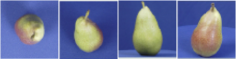
Using hand-held devices (such as mobile phones) to take multiangle shots around the apples in a natural-light environment, as shown in Figure 2, 50 images of each apple from different angles were retained, and each image was uniformly scaled to 512×512.
Figure 2. Multiangle images of an apple
The classification results on typical apple data sets are shown in Table 3. Through analyzing the experimental results, we can make two observations.
First, as expected, ACRMV achieved the best results due to the combination of feature representation and classification training. The ACRMV method based on multiviews is superior to the other three single-view methods because it integrates the information of multiple views.
Second, CCA only considers the correlation between different views and performs worse than the other methods.
The MVML-LA results are better than those of MISL on different data sets, which shows the effectiveness of considering the local structure. In addition, in the four tests for the different subsets of the training data, the four methods are seen to have similar advantages and disadvantages, which shows the consistency of the different methods.
Table 2. Statistical table for apple variety identification
|
Varieties |
Sample set |
Correction set |
Validation set |
|
Guoguang |
100 |
80 |
20 |
|
Fuji |
100 |
80 |
20 |
|
Wang Lin |
100 |
80 |
20 |
|
Jonagold |
100 |
80 |
20 |
|
Dounan |
100 |
80 |
20 |
|
Algorithm |
Fold1 |
Fold2 |
Fold3 |
Fold4 |
Average |
|
CCA |
86.14 |
87.01 |
87.24 |
88.57 |
87.24 |
|
MISL |
87.04 |
88.12 |
88.92 |
89.28 |
88.34 |
|
MVML-LA |
87.53 |
89.01 |
88.61 |
89.51 |
88.67 |
|
ACRMV-H |
87.34 |
87.51 |
87.93 |
89.28 |
88.02 |
|
ACRMV-L |
87.64 |
87.85 |
87.82 |
89.11 |
88.11 |
|
ACRMV-S |
88.01 |
88.57 |
88.34 |
90.15 |
88.77 |
|
ACRMV |
89.23 |
90.56 |
90.12 |
91.33. |
89.97 |
To further verify the effectiveness of the algorithm, in addition to the apple data set, three data sets are tested. The details are given below.
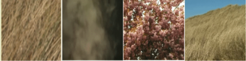
The dynamic texture refers to a continuous sequence of images that contains some static patterns in the time domain. The reason this kind of data is selected is that when classifying apples using red-green-blue (RGB) images, a large part of the surface texture of the apples plays a role. In the process of apple quality recognition, images from multiple angles provide a richer basis for quality recognition, and their data structures are similar to dynamic textures. Therefore, two common dynamic texture libraries, DynTex [26] and DynTex++ [27], are selected. DynTex contains three sub-datasets: DynTex-alpha contains 3 classes of 60 texture sequences, DynTex-beta contains 10 classes of 162 texture sequences, and DynTex-gamma contains 10 classes of 275 texture sequences. DynTex++ contains 36 classes, each with 100 texture sequences. A specific example is shown in Figure 3. For each sequence, subsequences with a length of 8 frames are constructed every 2 frames. LBP-TOP is used as the feature descriptor for each subsequence. Five texture sequences are selected as the training set for each class of the DynTex data set, and the rest constitute the test set. For DynTex++, half of the sequences of each class are selected as training sets and the rest as test sets.
The classification results are shown in Table 4.
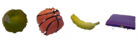
Apple variety identification can be summed up as an object identification task, so two object data sets are selected to assist algorithm testing. Both object databases contain multiangle pictures of an object. ETH-80 [28] consists of 8 objects, and each object contains 10 subclasses. The ratio of training and testing for each object is 1:1. The RGB-D [29] dataset contains 51 categories of objects. Each category of objects has more than 3 groups of photos. During training, 3 groups are randomly selected, and the rest constitute the test set. RGB-D also contains depth information, but only RGB information is used here. A specific example is shown in Figure 4.
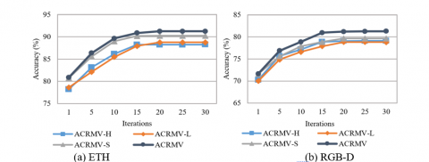
The dynamic texture recognition and object recognition tasks performed on the other two types of auxiliary data sets are shown in Tables 4 and 5. By analyzing the experimental results, we can see that in the two auxiliary classification tasks of dynamic texture classification and object recognition, the test results are similar to those on the apple data sets. ACRMV's strategy of multifeature fusion and joint training is superior to its corresponding single-view method and to the other multiview methods.
Figure 3. Examples of dynamic textures.
(a) ETH-80
(b) RGB-D
Figure 4. Examples of multiview objects
Table 4. Classification results of dynamic texture classification
|
Algorithm |
Alpha |
Beta |
Gamma |
Dyntex++ |
|
CCA |
83.01±6.48 |
80.14±4.74 |
80.25±4.14 |
88.40±0.32 |
|
MISL |
84.01±6.16 |
80.55±4.39 |
80.31±3.83 |
87.12±0.49 |
|
MVML-LA |
85.91±5.82 |
81.03±3.74 |
81.04±3.85 |
88.85±0.35 |
|
ACRMV-H |
82.17±6.41 |
80.12±3.66 |
77.93±4.50 |
88.37±0.71 |
|
ACRMV-L |
82.30±5.65 |
79.67±4.04 |
77.81±3.91 |
88.25±0.66 |
|
ACRMV-S |
85.21±6.03 |
80.91±3.93 |
79.84±4.04 |
89.74±0.47 |
|
ACRMV |
88.37±5.99 |
82.19±4.02 |
83.14±3.67 |
91.87±0.27 |
Table 5. Classification results of object categorization
|
Algorithm |
ETH |
RGB-D |
|
CCA |
89.17±4.94 |
78.23±3.55 |
|
MISL |
89.67±4.82 |
78.90±3.08 |
|
MVML-LA |
90.07±5.61 |
79.11±3.27 |
|
ACRMV-H |
88.25±5.06 |
79.09±2.65 |
|
ACRMV-L |
88.77±4.58 |
78.82±2.98 |
|
ACRMV-S |
90.25±4.02 |
79.65±2.15 |
|
ACRMV |
91.24±3.83 |
81.29±2.24 |
4.2 The effect of iterations on performance
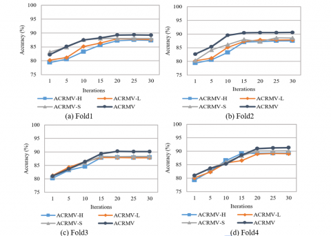
When optimizing the ACRMV algorithm in this paper, the feature representation and classifier weights are optimized by an alternating update strategy. As the number of iterations increases, the monitoring information not only affects the classifier learning but also indirectly guides the feature representation. To verify the influence of the number of iterations on performance, the change in the accuracy of ACRMV as the number of iterations increases is shown in Figure 5, and the following two trends can be seen:
First, with the increase in the number of iterations, both the single-view method and multiview method show improved accuracy. This is due to the combination of feature learning and classifier learning in ACRMV. Supervision information transmitted from the classification module can effectively improve feature learning. On the other hand, a highly discriminatory feature representation optimizes classifier learning.
Second, after approximately 15 iterations, the accuracy tends to be stable, which shows that the solution optimization algorithm can converge quickly. In addition, ACRMV with the multiview method has a slower convergence speed than the other three single-view methods, which shows that the information exchange between multiple views affects the convergence of the model to some extent, but it is also this sharing of information that makes the ACRMV result better than that of any single-view method. ACRMV achieves a good balance between convergence speed and accuracy.
Figure 5. The variation in accuracy with the number of iterations on the apple dataset
Similar to the classification accuracy analysis in section 3.2.1, the accuracy change and the convergence of the algorithm are still verified on four dynamic-texture data sets, and the relevant results are shown in Figure 6. Similar to the test results on the apple data set, ACRMV achieves the best results while balancing the convergence rate. Meanwhile, the SIFT feature view is still better than the LBP and HOG feature views, and the three feature views complement each other.
Finally, a comparative experiment with the same setup as above was carried out on two object data sets, and the results are shown in Figure 7.
Figure 6. The variation in the accuracy of dynamic-texture data sets with the number of iterations
Figure 7. The variation in the accuracy of multiangle object data sets with the number of iterations
Figure 8. Efficiency of the discriminant block selection algorithm
Figure 9. Result of three sets of multiview methods for discriminant image blocks
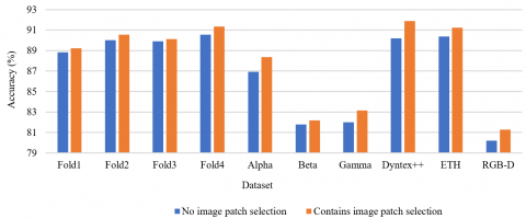
4.3 Validity of discriminant image block selection
One of the main reasons for the effectiveness of ACRMV is that it adopts a discriminant image block selection algorithm, which uses image blocks with higher discrimination as training data to reduce the impact of redundant data. To verify the effectiveness of this algorithm, the effect of the selection module is tested on 7 data sets individually. Figure 8 shows the relevant results. For all 7 data sets, the results when using the image block selection step are better than the results when this step is not performed.
4.4 Universality of discriminant image block selection
In addition, to further verify the generality of the image block selection step, an experiment is performed that combines this step with other multiview classification methods, such as CCA, MISL and MVML-LA. Figure 9 shows the comparison results of three multiview methods on the apple data set. The accuracy rate of the three methods is improved after the application of the sample selection module. Even CCA, which has weak performance among the three methods, after being combined with the module, shows a performance improvement result equivalent to that of the original MISL and MVML-LA methods.
In this paper, an apple category recognition method based on multiple views is proposed, which adopts the strategies of discrimination block selection and multiview fusion. The purpose of selecting the discrimination block is to remove redundant image areas by selecting representative image sub-blocks. In the multiview fusion step, shared subspace learning and classifier learning are integrated to take full advantage of feature representation and supervision information, thus achieving better results in apple variety identification and other tasks.
This work was supported by the Youth Foundation of Hebei Education Department (Grant No.: QN2018084), the Research and Practice Project of Higher Education Teaching Reform in Hebei Province (Grant No.: 2018GJJG121), the Introduction of Overseas Students Funded Projects in Hebei Province in 2019 (Grant No.: C20190342, C20190334), Science and Technology Foundation of Hebei Agricultural University (Grant No.: LG201814, LG201804), and Key research and development plan of Hebei Province (Grant No.: 20327401D).
[1] Ma, H.L., Wang, R.L., Cai, C., Wang, D. (2017). Rapid identification of apple varieties based on hyperspectral imaging. Transactions of the Chinese Society for Agricultural Machinery, 48: 305-312. https://doi.org/10.6041/j.issn.1000-1298.2017.04.040
[2] Yin, Y.B., Rao, X.Q., Ma, J.F. (2004). Methodology for nondestructive inspection of citrus maturity with machine vision. Transactions of The Chinese Society of Agricultural Engineering, 20(2): 144-147. https://doi.org/10.3321/j.issn:1002-6819.2004.02.034
[3] Liu, L., Qiao, X., Shi, X.D., Wang, Y., Shi, Y.G. (2019). Apple binocular visual identification and positioning system. Revue d'Intelligence Artificielle, 33(2): 133-137. https://doi.org/10.18280/ria.330208
[4] Xu, J. (2017). Study on classification of reticulate hami melon based on texture features. Zhejiang University.
[5] Wan, P., Toudeshki, A., Tan, H., Ehsani, R. (2018). A methodology for fresh tomato maturity detection using computer vision. Computers and Electronics in Agriculture, 146: 43-50. https://doi.org/10.1016/j.compag.2018.01.011
[6] Cubero, S., Alegre, S., Aleixos, N., Blasco, J. (2015). Computer vision system for individual fruit inspection during harvesting on mobile platforms. In Precision Agriculture'15, Wageningen Academic Publishers, pp. 3412-3419. http://dx.doi.org/10.3920/978-90-8686-814-8_68
[7] Cubero, S., Aleixos, N., Albert, F., Torregrosa, A., Ortiz, C., García-Navarrete, O., Blasco, J. (2014). Optimised computer vision system for automatic pre-grading of citrus fruit in the field using a mobile platform. Precision Agriculture, 15(1): 80-94. https://doi.org/10.1007/s11119-013-9324-7
[8] Cárdenas-Pérez, S., Chanona-Pérez, J., Méndez-Méndez, J.V., Calderón-Domínguez, G., López-Santiago, R., Perea-Flores, M.J., Arzate-Vázquez, I. (2017). Evaluation of the ripening stages of apple (Golden Delicious) by means of computer vision system. Biosystems Engineering, 159: 46-58. https://doi.org/10.1016/j.biosystemseng.2017.04.009.
[9] Zaborowicz, M., Boniecki, P., Koszela, K., Przybylak, A., Przybył, J. (2017). Application of neural image analysis in evaluating the quality of greenhouse tomatoes. Scientia Horticulturae, 218: 222-229. https://doi.org/10.1016/j.scienta.2017.02.001
[10] Cavallo, D.P., Cefola, M., Pace, B., Logrieco, A.F., Attolico, G. (2018). Non-destructive automatic quality evaluation of fresh-cut iceberg lettuce through packaging material. Journal of Food Engineering, 223: 46-52. https://doi.org/10.1016/j.jfoodeng.2017.11.042
[11] Moallem, P., Serajoddin, A., Pourghassem, H. (2017). Computer vision-based apple grading for golden delicious apples based on surface features. Information Processing in Agriculture, 4(1): 33-40. https://doi.org/10.1016/j.inpa.2016.10.003
[12] Kong, S., Fowlkes, C. (2017). Low-rank bilinear pooling for fine-grained classification. In Proceedings of the IEEE Conference on Computer Vision and Pattern Recognition, pp. 365-374. https://doi.org/10.1109/CVPR.2017.743
[13] Reed, S., Akata, Z., Lee, H., Schiele, B. (2016). Learning deep representations of fine-grained visual descriptions. In Proceedings of the IEEE Conference on Computer Vision and Pattern Recognition, pp. 49-58. https://doi.org/10.1109/CVPR.2016.13
[14] Zhao, J., Xie, X., Xu, X., Sun, S. (2017). Multi-view learning overview: Recent progress and new challenges. Information Fusion, 38: 43-54. https://doi.org/10.1016/j.inffus.2017.02.007
[15] Kumar, A., Rai, P., Daume, H. (2011). Co-regularized multi-view spectral clustering. In Advances in Neural Information Processing Systems, pp. 1413-1421.
[16] Hardoon, D.R., Szedmak, S., Shawe-Taylor, J. (2004). Canonical correlation analysis: An overview with application to learning methods. Neural computation, 16(12): 2639-2664. https://doi.org/10.1162/0899766042321814
[17] Xia, R., Pan, Y., Du, L., Yin, J. (2014). Robust multi-view spectral clustering via low-rank and sparse decomposition. In Twenty-Eighth AAAI Conference on Artificial Intelligence, pp. 352–360.
[18] Lu, C., Feng, J., Lin, Z., Mei, T., Yan, S. (2018). Subspace clustering by block diagonal representation. IEEE Transactions on Pattern Analysis and Machine Intelligence, 41(2): 487-501. https://doi.org/10.1109/tpami.2018.2794348
[19] Xu, C., Tao, D., Xu, C. (2015). Multi-view intact space learning. IEEE Transactions on Pattern Analysis and Machine Intelligence, 37(12): 2531-2544. https://doi.org/10.1109/tpami.2015.2417578
[20] Zhao, Y., You, X., Yu, S., Xu, C., Yuan, W., Jing, X.Y., Zhang, T.P., Tao, D. (2018). Multi-view manifold learning with locality alignment. Pattern Recognition, 78: 154-166. https://doi.org/10.1016/j.patcog.2018.01.012
[21] Tian, Y., Fan, B., Wu, F. (2017). L2-Net: Deep learning of discriminative patch descriptor in euclidean space. In Proceedings of the IEEE Conference on Computer Vision and Pattern Recognition, pp. 661-669. http://dx.doi.org/10.1109/CVPR.2017.649
[22] Singh, S., Gupta, A., Efros, A.A. (2012). Unsupervised discovery of mid-level discriminative patches. In European Conference on Computer Vision, pp. 73-86. http://dx.doi.org/10.1007/978-3-642-33709-3_6
[23] Huang, J., Zhang, T., Metaxas, D. (2011). Learning with structured sparsity. Journal of Machine Learning Research, 12(11): 3371-3412. http://dx.doi.org/10.1145/1553374.1553429
[24] Boyd, S., Parikh, N., Chu, E. (2011). Distributed optimization and statistical learning via the alternating direction method of multipliers. Foundations and Trends® in Machine Learning, 3(1): 1-122. http://dx.doi.org/10.1561/2200000016
[25] Bach, F., Jenatton, R., Mairal, J., Obozinski, G. (2012). Structured sparsity through convex optimization. Statistical Science, 27(4): 450-468. http://dx.doi.org/10.1214/12-sts394
[26] Péteri, R., Fazekas, S., Huiskes, M.J. (2010). DynTex: A comprehensive database of dynamic textures. Pattern Recognition Letters, 31(12): 1627-1632. https://doi.org/10.1016/j.patrec.2010.05.009
[27] Ghanem, B., Ahuja, N. (2010). Maximum margin distance learning for dynamic texture recognition. In European Conference on Computer Vision, pp. 223-236. http://dx.doi.org/10.1007/978-3-642-15552-9_17
[28] Leibe, B., Schiele, B. (2003). Analyzing appearance and contour based methods for object categorization. In 2003 IEEE Computer Society Conference on Computer Vision and Pattern Recognition, Madison, WI, USA, USA, II-409. http://dx.doi.org/10.1109/CVPR.2003.1211497
[29] Lai, K., Bo, L., Ren, X., Fox, D. (2011). A large-scale hierarchical multi-view RGB-D object dataset. In 2011 IEEE International Conference on Robotics and Automation, pp. 1817-1824. http://dx.doi.org/10.1109/ICRA.2011.5980382