Hui Lu | Tichun Wang*
OPEN ACCESS
In recent years, the prediction of automobile noise has attracted much attention from the academia. This paper aims to develop an automobile noise prediction model based on basic vehicle parameters and vehicle speed, rather than the features calculated from noise data. First, the extension data mining (EDM) was adopted to preprocess the original data, select the features and establish the matter-element models of automobile noise. Then, the extremum entropy method (EEM), an improved information entropy method, was selected to determine the weight of each feature for the calculation of comprehensive correlation function. To verify its effectiveness of the proposed model, our model was applied to experiments on an automobile noise dataset, in comparison with logistic regression and decision tree. The results show that our model outperformed the contrastive methods in prediction accuracy, eliminating the need to set hyper-parameters in advance. The research findings provide a new method to predict automobile noise based on basic vehicle parameters and vehicle speed.
automobile noise prediction, extension data mining (EDM), weight calculation, information entropy
In recent years, the automobile industry has raised much concern over the noise, vibration and harshness (NVH) problem. In addition to vibration noise, the noise in automobile may arise from the engine assembly, the exhaust system, the transmission system, and the driving system when the vehicle starts and drives. Excessive automobile noise degrades the driving experience, and harms the physical and mental health of the driver. Long-term exposure to automobile noise will lead to physical illnesses like tinnitus, dreaminess, palpitation and irritability, hearing loss and even deafness. Therefore, many acoustic models [1-10] have been developed to measure and predict automobile noise.
On acoustic measurement, there are many widely used numerical and test methods. For example, D.V. Nehete et al. [11] improved the coupled finite-element model based on the frequency response function of acoustic vibration, solving the uncertainty of the stiffness and damping and acoustic cavity in the original model. Modak [12] developed a formulation for direct updating of mass and stiffness matrices of the acoustic and structural domains of a coupled vibro-acoustic model. To identify interior noise sources, Huang et al. [13] developed a partial wavelet coherence analysis method with a time-frequency partial coherence function, in which the instantaneous phase relationship between the noise source and the receiving point is obtained through wavelet transform and partial coherence analysis.
On acoustic prediction, intelligence algorithms have been extensively adopted for predicting the acoustic quality of automobile. For instance, Huang et al. [14] proposed regression-based deep belief networks (DBNs) to predict the interior sound quality, showing a better accuracy and robustness of the method. He et al. [15] applied the support vector machine (SVM) to predict the interior acoustic quality of the accelerating vehicle, and proved that the SVM prediction model outperforms the multiple linear regression (MLR) model in reflecting the nonlinear mapping between objective evaluation parameters and subjective irritability. Xu et al. [16] introduced particle swarm optimization (PSO) to improve the prediction accuracy of the SVM prediction model. With the aid of the PSO, Zhang et al. [17] optimized the initial weights and neuron thresholds of the prediction model based on backpropagation neural network (BPNN). Wang et al. [18] combined the finite-element method (FEM) with artificial neural network (ANN) to predict the acoustic behavior of a human auditory system. Ahmed et al. [19] proposed a neural network (NN) model to predict and simulate the propagation of vehicular traffic noise in a dense residential area, which was verified to be a promising tool for traffic noise assessment in dense urban areas. Song [20] set up an acoustic quality prediction model based on principal component analysis (PCA) and least squares support vector machine (LSSVM), which outputs the subjective irritability based on the objective parameters of automobile noise obtained by the PCA, and verified that the combined method can predict the quality of interior noise when the vehicle is in unsteady conditions. Huang [21] designed an intelligent acoustic model based on a deep neural network (DNN) called the Laplacian score-deep belief network (LS-DBN), and demonstrated the good prediction ability of the model for interior noise quality of electric vehicles (EVs). Lisa S. [22] proposed 150 ANN models with different hidden layers to predict automobile noise.
In general, the existing models predict the subjective perception of noise quality, in the light of the objective parameters computed from the sound data. None of them considers the basic parameters of the vehicle or the vehicle speed. To make up for the gap, this paper develops an automobile noise prediction model, using the basic vehicle parameters and vehicle speed, based on the extension data mining (EDM) algorithm).
The remainder of this paper is organized as follows: Section 2 and Section 3 introduce the EDM algorithm and the weight calculation method, respectively; Section 4 presents the proposed prediction model of automobile noise; Section 5 verifies the efficiency of our model through an experiment, and compares the results of our model with those of logistics regression and decision tree; Section 6 wraps up this paper with meaningful conclusions.
2.1 Extension theory
Extension theory mainly includes matter-element theory and extension set theory. To formally describe things, the 1D matter-element model, which consists of things, features and values of features, can be defined as:
$M=(\text { things, features, values })=(O, C, V)$ (1)
where, O is the name of a matter; C is the feature of the matter; and V is the value of the feature.
If the value of the feature has a classical domain or a range, the matter-element model can be rewritten as:
$M=(O, C, V)=(O, C,\langle a, b\rangle)$ (2)
where, a and b are the upper and lower bounds of the classical domain, respectively.
Because the real-world objects often have multiple features, the multi-dimensional matter-element can be designated as:
$M=\left[\begin{array}{ccc}{O,} & {C_{1},} & {V_{1}} \\ {} & {C_{2},} & {V_{2}} \\ {} & {\vdots} & {\vdots} \\ {} & {C_{n},} & {V_{n}}\end{array}\right]$ (3)
Then, the extension set is needed to realize the dynamic classification of things. The extension set can determine the changes of things both quantitatively and qualitatively. Meanwhile, the matter-element model can describe the internal structure, relationship and changing state of things in natural and social phenomena in a rational manner. Overall, the extension theory offers an effective tool to describe the variability of things.
2.2 EDM algorithm
The EDM relies on the extension theory to overcome the defect of traditional data mining: the knowledge cannot be mined under variable conditions. First, the matter-element model is adopted to describe the data, forming a new data representation for further transform. Then, the transform law is derived from the results of comprehensive correlation function, and labeled as the extension knowledge.
The process of the EDM algorithm can be summed up as four steps:
Step 1. Obtain the joint domains and classical domains of each feature to establish the matter-element models.
In extension theory, the matter-element model is defined as $M=(O, C, V),$ where $O$ is the name of a matter, $C$ is the feature of the matter and $V$ is the value of the feature. The matter-element model of a particular thing can be defined as:
$M_{i}=\left[\begin{array}{ccc}{O_{i},} & {C_{1},} & {V_{i 1}} \\ {} & {C_{2},} & {V_{i 2}} \\ {} & {\vdots} & {\vdots} \\ {} & {C_{n},} & {V_{i n}}\end{array}\right]=\left[\begin{array}{ccc}{O_{i},} & {C_{1},} & {\left\langle a_{i 1}, b_{i 1}\right\rangle} \\ {} & { C_{2},} & {\left\langle a_{i 2}, \mathbf{b}_{i 2}\right\rangle} \\ {} & {\vdots} & {\vdots} \\ {} & { C_{n},} & {\left\langle a_{i n}, \mathbf{b}_{m}\right\rangle}\end{array}\right]$ (4)
where $a_{i}$ and $b_{i}$ are the lower and upper bounds of $V$ respectively.
Let $O_{U}$ be the set of matter-element models, and $V_{U n}=$ $\left\langle a_{U n}, b_{U n}\right\rangle \subset V_{i n .}$ Then, the joint domains can be constructed as:
$M_{U}=\left[\begin{array}{ccc}{O_{U},} & {C_{1},} & {V_{U 1}} \\ {} & {C_{2},} & {V_{U 2}} \\ {} & {\vdots} & {\vdots} \\ {} & {C_{n},} & {V_{U n}}\end{array}\right]=\left[\begin{array}{ccc}{O_{U},} & {C_{1},} & {\left\langle a_{U 1}, \mathrm{b}_{U_{1}}\right\rangle} \\ {} & { C_{2},} & {\left\langle a_{U_{2}}, \mathrm{b}_{U_{2}}\right\rangle} \\{} & {\vdots} & {\vdots} \\ {} & { C_{n},} & {\left\langle a_{U_{n}}, \mathrm{b}_{U_{n}}\right\rangle}\end{array}\right]$ (5)
Step 2. Calculate the correlation function.
According to the extension theory, the correlation function can objectively quantify the correlation degree of each feature, and identify the process of quantitative and qualitative changes.
Let $X_{0}=<a_{0}, b_{0}>$ and $X=<a, b>, X_{0} \subseteq X$ be the optimal range and the range of a feature, respectively. Then, the element $x$ between $X_{0}$ and $X$ can be defined as:
$D\left(x, X_{0}, X\right)=\left\{\begin{array}{l}{a-b, \rho\left(x, X_{0}\right)=\rho(x, X)} \\ {\rho\left(x, X_{0}\right)-\rho(x, X), \rho\left(x, X_{0}\right) \neq \rho(x, X), x \notin X_{0}} \\ {\rho\left(x, X_{0}\right)-\rho(x, X)+a-b, \rho\left(x, X_{0}\right) \neq \rho(x, X), x \in X_{0}}\end{array}\right.$ (6)
where, $\rho\left(x, X_{0}\right)$ is the extension distance between $x$ and the optimal range $X_{0}:$
$\rho\left(x, X_{0}\right)=\left|x-\frac{a+b}{2}\right|-\frac{b-a}{2}$ (7)
Assuming that the optimum value appears at the midpoint of the range, then the correlation degree $k$ of $x$ can be computed as:
$k(x)=\left\{\begin{array}{l}{\frac{\rho(x, X)}{D\left(x, X_{0}, X\right)}-1, \rho\left(x, X_{0}\right)=\rho(x, X)} \\ {\frac{\rho(x, X)}{D\left(x, X_{0}, X\right)}, \text { else }}\end{array}\right.$ (8)
If $k(x) \geq 0,$ it reflects the degree to which $x$ belongs to $X_{0}$ otherwise, it reflects the degree to which $x$ does not belong to $X_{0} ;$ if $-1<k(x)<0,$ it is an extension domain, i.e. $x$ still has a chance to become an element of the classical domain after some transforms.
Step 3. Compute the comprehensive correlation function.
The comprehensive correlation function illustrates the correlation degrees between the samples and the classes. The greater the correlation degree, the more likely it is for a sample to belong to a class.
For a sample $X=\left(x_{1}, x_{2}, \cdots, x_{n}\right),$ the comprehensive correlation function $K_{i}(X)$ can be expressed as:
$K_{i}(X)=\sum_{j=1}^{n} \omega_{j} k_{j}\left(x_{j}\right)$ (9)
where, $\omega_{j}$ is the weight of the $j$ -th feature of the sample; $\sum_{j=1}^{n} \omega_{j}=1, k_{j}\left(x_{j}\right)$ is the correlation degree between the $j$ -th feature and its value.
Step $4 .$ Predict the value of $X$ according to the highest comprehensive correlation degree.
The weight of each feature should be calculated accurately, because the prediction result depends heavily on the weights of different features. In general, feature weights are computed by expert scoring, binary comparison, analytic hierarchy process (AHP) and fuzzy statistics. For objectivity, this paper chooses to calculate the weight of each feature based on information entropy method. Note that the entropy value represents the relative importance of each feature, rather than the amount of actual information [23].
Currently, there are five information entropy methods improved by dimensionless strategies, namely, normalized translational entropy method (NTEM), extremum entropy method (EEM), linear proportional entropy method (LPEM), vector gauge entropy method (VGEM) and efficacy coefficient entropy method (ECEM). The NTEM and the EEM stand out for their high calculation accuracy [24]. However, the value of zero may appear in the process of NTEM, in which the data is normalized and translated instead of being used directly. Thus, this paper decides to compute the weight of each feature by the EEM.
The EMM-based weight calculation is implemented in four steps:
Step 1. Normalize the data matrix X.
For a dataset of $m$ samples and $n$ features, let $x_{i j}$ be the $j$ -th feature of the $i$ -th sample. Then, the dataset can be written as a data matrix below:
$X=\left[\begin{array}{cccc}{x_{11}} & {x_{12}} & {\cdots} & {x_{1 n}} \\ {x_{21}} & {x_{22}} & {\cdots} & {x_{2 n}} \\ {\vdots} & {\vdots} & {} & {\vdots} \\ {x_{m 1}} & {x_{m 2}} & {\cdots} & {x_{m n}}\end{array}\right]$ (10)
Considering the dimensional difference among the features, the data matrix X can be normalized by:
$r_{i j}=\frac{x_{i j}-m_{j}}{M_{j}-m_{j}}$ (11)
where, $M_{j}=\max _{j}\left\{x_{i j}\right\} ; m_{j}=\min _{j}\left\{x_{i j}\right\}$.
Step 2. Compute the entropy of the j-th feature in automobile noise:
$p_{i j}=\frac{r_{i j}}{\sum_{i=1}^{n} r_{i j}}=\frac{x_{i j}-m_{j}}{\sum_{i=1}^{n}\left(x_{i j}-m_{j}\right)}$ (12)
$E_{j}=-\frac{1}{\ln m} \sum_{i=1}^{m} p_{i j} \ln p_{i j}$ (13)
where, $k=\frac{1}{\ln m}$ is the normalization coefficient; the negative sign “-” is to keep the entropy positive.
Step 3. Compute the deviation degree of each feature.
As shown in Equation $(12),$ the $E_{j}$ value of a given feature is negatively correlated with the difference of $x_{i j} .$ If all the $x_{i j}$ are equal, then $E_{j}=E_{\max }=1,$ indicating that feature $x_{j}$ has no impact on the evaluation object. The greater the difference of $x_{i j},$ the smaller the value of $E_{j},$ and the more important feature $x_{j}$ is to the evaluation object. Thus, the deviation degree $d_{j}$ of the $j$ -th feature can be defined as:
$d_{j}=1-E_{j}$ (14)
The greater the value of dj, the more important the j-th feature is.
Step 4. Obtain the weight of each feature by:
$\omega_{j}=\frac{d_{j}}{\sum_{j=1}^{n} d_{j}}=\frac{1-E_{j}}{\sum_{j=1}^{n}\left(1-E_{j}\right)}$ (15)
Figure 1. The workflow of our model
In this paper, the EDM algorithm and the EEM are integrated into a novel efficient prediction model for automobile noise. As shown in Figure 1, our model involves the following steps:
Step 1. Select the main influencing factors of automobile noise.
A total of 13 features were selected as the model inputs to effectively predict the automobile noise, according to the basic parameters of the vehicle and the vehicle speed. The selected features include engine capacity, the number of engine cylinders, the number of valves per cylinder of engine, the total number of engine valves, engine torque, vehicle weight, vehicle length, vehicle width, vehicle height, wheel base, capacity of fuel tank, and engine power. All the features are expressed as numerical data.
Step 2. Preprocess the data.
The original data were cleaned and transformed into forms recognizable by machine language. The incomplete, noisy and inconsistent data were corrected by filling in missing values, smoothing noise and identifying outliers. Then, the data were subjected to generalization, normalization and attribute reconstruction, and thus converted to a form suitable for data mining.
The input data are normalized by:
$x_{i j}=\frac{x_{i j}-\overline{x_{j}}}{\max x_{j}-\min x_{j}}$ (16)
Step 3. Calculate the classical domains and joint domains of each feature, and construct the matter-element models of automobile noise.
Traditionally, the classical domains and the joint domains are calculated by the statistical method. In this paper, the classical domains are set according to lower and upper bounds of field-test records, and the joint domains are obtained by the three-sigma rule based on classical domains. Specifically, the mean $\mu_{i j}$ and variance $\sigma_{i j}$ of features were obtained through data mining, while the corresponding joint domain was established according to the three-sigma rule in the normal distribution theory, that is, 99.7% of the data in the normal distribution fall within $<\mu_{i j}-3 \sigma_{i j}, \mu_{i j}+3 \sigma_{i j}>$.
Next, the automobile noise was divided into 4 levels based on the hearing of normal people. Level 0 noise is less than 40dB, signifying a relatively quiet interior environment. Level 1 noise lies between 40 and 60dB, meaning that the interior environment has a moderate level of noise. Level 2 noise belongs to the interval between 60dB and 70 dB. On this level, the interior environment is full of noise that may harm our nerves. Level 3 noise is greater than 80dB, when the interior environment is so noisy that the passenger may suffer from damages in their nerve cells.
Hence, the matter-element model of the i-th noise level can be established as:
$M_{i}=\left(\mathrm{O}_{i}, \mathrm{C}, x\right)=\left(\begin{array}{ccc}{\text { Noise level } i,} & {\text { Engine capacity },} & {V_{i1}} \\ {} & {\text { The number of engine cylinders, }} & {V_{i2}} \\ {} & {\vdots} & {\vdots} \\ {} & {\text { Speed }} & {V_{13}}\end{array}\right)$ (17)
Step 5. Calculate the feature weights of each matter-element model by Equations (10)-(15).
Step 6. Import the sample Xi to be predicted.
Step 7. Calculate the correlation function by Equations (6)-(8).
Step 8. Compute the comprehensive correlation function by Equation (9).
Step 9. Predict the noise level of Xi, rank the comprehensive evaluation value, and take the highest value as the predicted noise level.
Our model was verified through experiments on an automobile noise dataset (https://www.kaggle.com/murtio/car-noise-specification). The original dataset contains 1,895 samples with 72 features. Here, the dataset is divided into a training set and a testing set at the ratio of 9:1.
5.1 Model construction
First, the original data were preprocessed to remove the features with lots of missing values and the semantically duplicate features (e.g. engine power in horsepower and engine power in kilowatt), and to delete categorical features like automobile manufacturers and models. Then, the 13 features mentioned before were selected as the inputs of our model: engine capacity $\left(c_{1}\right) /\left(\mathrm{cm}^{3}\right),$ the number of engine cylinders $\left(c_{2}\right),$ the number of valves per cylinder of engine $\left(c_{3}\right)$ the total number of engine valves $\left(c_{4}\right),$ engine torque $\left(c_{5}\right) /(\mathrm{N}$. $\mathrm{m}$ ), vehicle weight $\left(c_{6}\right) /(\mathrm{kg}),$ vehicle length $\left(c_{7}\right) /(\mathrm{mm})$ vehicle width $\left(c_{8}\right) /(\mathrm{mm}),$ vehicle height $\left(c_{9}\right) /(\mathrm{mm}),$ wheel base $\left(c_{10}\right) /(\mathrm{mm}),$ capacity of fuel $\operatorname{tank}\left(c_{11}\right),$ engine power $\left(c_{12}\right) /(\mathrm{kW}),$ and speed $\left(c_{13}\right) /\left(\mathrm{km} \cdot \mathrm{h}^{-1}\right) .$ Next, the automobile noise was divided into 4 levels. Through preprocessing, the authors obtained 3,180 samples with 13 features and 4 class labels.
The classical domains were obtained from the training set normalized by Eq. (13). The information entropy method was used to calculate the weights of the 13 features under each noise level. Table 1 presents the weights and the classical domains of the 13 features at each noise level.
Table 1. Weights and classical domains of the 13 features at each noise level
|
|
O0 |
O1 |
O2 |
O3 |
||||
|
Weight |
Classical domain |
Weight |
Classical domain |
Weight |
Classical domain |
Weight |
Classical domain |
|
|
c1 |
0.093 |
<1149,4969> |
0.073 |
<996,7000> |
0.070 |
<996,8285> |
0.070 |
<996,8285> |
|
c2 |
0.019 |
<4,8> |
0.072 |
<3,12> |
0.071 |
<3,12> |
0.080 |
<3,10> |
|
c3 |
-0.029 |
<2,4> |
0.058 |
<2,5> |
0.057 |
<2,5> |
-0.003 |
<2,4> |
|
c4 |
0.103 |
<8,32> |
0.076 |
<6,48> |
0.075 |
<6,48> |
0.076 |
<6,40> |
|
c5 |
0.110 |
<82,522> |
0.083 |
<82,856> |
0.083 |
<82,856> |
0.092 |
<82,856> |
|
c6 |
0.111 |
<966,2537> |
0.085 |
<785,2684> |
0.085 |
<785,2684> |
0.009 |
<785,2684> |
|
c7 |
0.112 |
<3713,5820> |
0.090 |
<2695,6350> |
0.089 |
<2695,6350> |
0.100 |
<2695,6350> |
|
c8 |
0.084 |
<1500,2165> |
0.084 |
<1410,2624> |
0.083 |
<1410,2624> |
0.095 |
<1410,2624> |
|
c9 |
0.097 |
<1400,1910> |
0.092 |
<1150,2000> |
0.091 |
<1150,2000> |
0.103 |
<1150,2000> |
|
c10 |
0.108 |
<2466,3560> |
0.085 |
<1867,4080> |
0.085 |
<1867,4080> |
0.091 |
<1867,4080> |
|
c11 |
0.113 |
<35,98> |
0.083 |
<30,132> |
0.082 |
<30,132> |
0.092 |
<30,132> |
|
c12 |
0.108 |
<44,327> |
0.074 |
<40,487> |
0.073 |
<40,487> |
0.072 |
<40,487> |
|
c13 |
-0.029 |
0 |
0.047 |
<0,120> |
0.056 |
<0,140> |
0.033 |
<80,120> |
5.2 Random sample experiment
A random sample was taken from the testing set. The initial and normalized forms of the sample can be respectively expressed as:
$M_{x}=\left(\mathrm{O}_{x}, \mathrm{C}, x\right)=\left[\begin{array}{ccc}{O_{x},} & {c_{1},} & {3000} \\ {} & {c_{2},} & {6} \\ {}& {c_{3},} & {4} \\{}& {c_{4},} & {24} \\{}& {c_{5},} & {440} \\ {}& {c_{6}} & {1769}\\ {}& {c_{7}} & {4623}\\ {}& {c_{8}} & {1864}\\ {}& {c_{9}} & {1483}\\ {}& {c_{10}} & {2776}\\ {}& {c_{11}} & {67}\\{}& {c_{12},} & {224} \\{}& {c_{13},} & {0} \end{array}\right]$ (18)
$M_{x}=\left(\mathrm{O}_{x}, \mathrm{C}, x\right)=\left[\begin{array}{ccc}{O_{x},} & {c_{1},} & {0.193} \\ {} & {c_{2},} & {0.222} \\ {}& {c_{3},} & {0.667} \\{}& {c_{4},} & {0.333} \\{}& {c_{5},} & {0.438} \\ {}& {c_{6}} & {0.584}\\ {}& {c_{7}} & {0.354}\\ {}& {c_{8}} & {0.341}\\ {}& {c_{9}} & {0.422}\\ {}& {c_{10}} & {0.392}\\ {}& {c_{11}} & {0.256}\\{}& {c_{12},} & {0.125} \\{}& {c_{13},} & {0} \end{array}\right]$ (19)
After that, the comprehensive correlation degrees of the sample to each noise level were calculated by Eq. (6). The calculation results are shown in Table 2.
The results show that the comprehensive correlation degree of the sample peaked at 0.961, corresponding to the noise level ranked at the 1st place. The prediction is obviously correct.
The remaining 317 test samples were predicted in the same way. The final results of the experiment are shown in Figure 2, where the true and predicted noise levels of the testing set are displayed as red star lines and blue cross lines, respectively. It can be seen that the model sometimes predicts level 1 to level 0, and level 3 to level 2 incorrectly. This means the model has difficulty in differentiating between adjacent noise levels. The reason might be that the classical domains of some features are totally identical or partially overlapping for the adjacent noise levels.
Table 2. Comprehensive correlation degrees of the sample and each noise level
|
Noise level |
Comprehensive correlation degree |
Rank |
|
0 |
0.528 |
2nd |
|
1 |
0.961 |
1st |
|
2 |
-0.241 |
3rd |
|
3 |
-0.667 |
4th |
Figure 2. Prediction results of our model for automobile noise level
Based on the prediction results, 7 features with significant impact on automobile noise were determined: total number of engine valves $\left(c_{4}\right),$ engine torque $\left(c_{5}\right),$ vehicle weight $\left(c_{6}\right)$ vehicle length $\left(c_{7}\right),$ vehicle height $\left(c_{9}\right),$ wheel base $\left(c_{10}\right)$ and capacity of fuel $\operatorname{tank}\left(c_{11}\right) .$ The value of all these features is positively correlated with the level of automobile noise.
5.3 Comparative experiments
Using the same dataset, logistic regression and decision tree were also applied to predict the automobile noise level. Then, their error rates were compared with that of our method through 10-fold cross validation (Table 3).
For the logistic regression, the regularization parameter was denoted as L2, and the training set was normalized by equation (5). The noise levels predicted by this method are shown in Figure 3. It can be seen that the samples marked as level 0 are all wrong predictions, possibly due to the small number of level 0 noise samples in the training set.
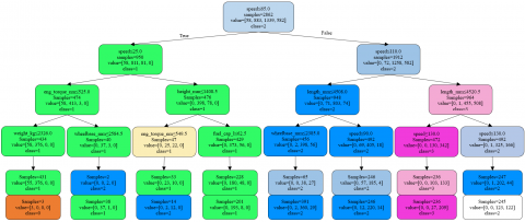
For the decision tree (Figure 4), the split node evaluation index was set as information gain, and the maximum depth of tree was set to 4. The prediction results in Figure 4 show that the decision tree achieved better prediction of level 0 samples.
Figure 3. Prediction results of logistic regression for automobile noise level
Figure 4. Prediction results of decision tree for automobile noise level
Figure 5. Visualization of decision tree
As shown in Table 3, the proposed EDM, logistic regression and decision tree had an error rate of 17.30%, 22.64%, and 21.07%. Obviously, our model achieved the highest prediction accuracy. Compared with the contrastive methods, our model does not need to set any hyper-parameter, and could obtain varying extension knowledge rather than fixed knowledge. However, the performance of our model depends on the scale of the data. If the data is too large, it would be too tedious to build the matter-element models.
Table 3. Error rates of the three models
|
Model |
Error rate |
|
EDM |
17.30% |
|
Logistic regression |
22.64% |
|
Decision tree |
21.07% |
This paper combines the extension theory and data mining to solve the knowledge mining problem based on big data, and demonstrates that the combined method is excellent in expressing the problem quantitatively and formally. Specifically, an EDM-based model was established to predict automobile noise according to basic vehicle parameters and vehicle speed. First, the original data were preprocessed, the features were selected, and the matter-element models of automobile noise were constructed. Then, the EEM was adopted to determine the weight of each feature for the comprehensive correlation function of noise. The noise level corresponding to the highest comprehensive correlation degree of the sample was taken as the prediction result. Finally, the excellence of our model was proved through comparative experiments against logistic regression and decision tree. The future research will further improve the feature selection process of our model.
This research is supported by the National Natural Science Foundation of China (Grant No.: 51775272 and 51005114), and the Domestic Visiting and Training Program for Outstanding Young Talents in Colleges and Universities of Anhui Province, China (Grant No.: gxgnfx2019150).
[1] Ma, C., Chen, C., Liu, Q., Gao, H., Li, Q., Gao, H., Shen, Y. (2017). Sound quality evaluation of the interior noise of pure electric vehicle based on neural network model. IEEE Transactions on Industrial Electronics, 64(12): 9442-9450. https://doi.org/10.1109/TIE.2017.2711554
[2] Sarafraz, H., Sarafraz, Z., Hodaei, M., Sayeh, M. (2016). Minimizing vehicle noise passing the street bumps using genetic algorithm. Applied Acoustics, 106: 87-92. https://doi.org/10.1016/j.apacoust.2015.11.021
[3] Le, D.C., Zhang, J., Pang, Y. (2018). A bilinear functional link artificial neural network filter for nonlinear aruhctive noise control and its stability condition. Applied Acoustics, 132: 19-25. https://doi.org/10.1016/j.apacoust.2017.10.023
[4] Huang, H.B., Li, R. X., Yang, M.L., Lim, T.C., Ding, W.P. (2017). Evaluation of vehicle interior sound quality using a continuous restricted Boltzmann machine-based DBN. Mechanical Systems and Signal Processing, 84: 245-267. https://doi.org/10.1016/j.ymssp.2016.07.014
[5] Lin, F., Zuo, S., Deng, W., Wu, S. (2017). Noise prediction and sound quality analysis of variable-speed permanent magnet synchronous motor. IEEE Transactions on Energy Conversion, 32(2): 698-706. https://doi.org/10.1109/TEC.2017.2651034
[6] Huang, H.B., Huang, X.R., Li, R. X., Lim, T.C., & Ding, W.P. (2016). Sound quality prediction of vehicle interior noise using deep belief networks. Applied Acoustics, 113: 149-161. https://doi.org/10.1016/j.apacoust.2016.06.021
[7] Alessandro, Z. (2019). Full field optical measurements in experimental modal analysis and model updating. Journal of Sound and Vibration, 442: 817-842. https://doi.org/10.1016/j.jsv.2018.09.048
[8] Huang, H.B., Li, R.X., Huang, X.R., Lim, T.C., Ding, W.P. (2016). Identification of vehicle suspension shock absorber squeak and rattle noise based on wavelet packet transforms and a genetic algorithm-support vector machine. Applied Acoustics, 113: 137-148. https://doi.org/10.1016/j.apacoust.2016.06.016
[9] Antonio, P., Laurent, B., Karl, J., Domenico, M., Wim, D. (2018). The measurement of gear transmission error as an NVH indicator: Theoretical discussion and industrial application via low-cost digital encoders to an all-electric vehicle gearbox. Mechanical Systems and Signal Processing, 110: 368-389. https://doi.org/10.1016/j.ymssp.2018.03.005
[10] Pallas, M.A., Michel, B., Roger, C., Martin, C., Marco, C., Matthew, M. (2016). Towards a model for electric vehicle noise emission in the European prediction method CNOSSOS-EU. Applied Acoustics, 113: 89-101. https://doi.org/10.1016/j.apacoust.2016.06.012
[11] Nehete, D.V., Modak, S.V., Gupta, K. (2016). Coupled vibro-acoustic model updating using frequency response functions. Mechanical Systems and Signal Processing, 70: 308-319. https://doi.org/10.1016/j.ymssp.2015.09.002
[12] Modak, S.V. (2014). Direct matrix updating of vibro-acoustic finite element models using modal test data. AIAA Journal, 52(7): 1386-1392. https://doi.org/10.2514/1.J052558
[13] Huang, H.B., Huang, X. R., Yang, M.L., Lim, T.C., Ding, W.P. (2018). Identification of vehicle interior noise sources based on wavelet transform and partial coherence analysis. Mechanical Systems and Signal Processing, 109: 247-267. https://doi.org/10.1016/j.ymssp.2018.02.045
[14] Huang, H.B., Huang, X. R., Li, R.X., Lim, T.C., Ding, W.P. (2016). Sound quality prediction of vehicle interior noise using deep belief networks. Applied Acoustics, 113: 149-161. http://dx.doi.org/10.1016/j.apacoust.2016.06.021
[15] He, Y.S., Tu, L.E., Xu, Z.M., Zhang, Z.F., Xie, Y.Y. (2015). The application of support vector machine to the prediction of vehicle interior sound quality during acceleration. Automotive Engineering, 37(11): 1328-1333. https://doi.org/10.19562/j.chinasae.qcgc.2015.11.016
[16] Xu, Z.M., Xie, Y.Y., He, Y.S. (2015). Evaluation of car interior sound quality based on PSO-SVM. Journal of Vibration and Shock, 34(2): 25-29. https://doi.org/10.13465/j.cnki.jvs.2015.02.005
[17] Zhang, E.L., Hou, L., Shen, C., Shi, Y.L., Zhang, Y.X. (2016). Sound quality prediction of vehicle interior noise and mathematical modeling using a back propagation neural network (BPNN) based on particle swarm optimization. Measurement Science and Technology, 27: 015801. https://doi.org/10.1088/0957-0233/27/1/015801
[18] Wang, Y.S., Guo, H., Feng, T.P., Ju, J., Wang, X.L. (2017). Acoustic behavior prediction for low-frequency sound quality based on finite element method and artificial neural network. Applied Acoustics, 122: 62-71. https://doi.org/10.1016/j.apacoust.2017.02.009
[19] Ahmed, A.A., Biswajeet P. (2019). Vehicular traffic noise prediction and propagation modelling using neural networks and geospatial information system. Environ Monit Assess, 191: 190. https://doi.org/10.1007/s10661-019-7333-3
[20] Song, W.B., Zuo, Y.Y. (2019). Prediction of HEV interior sound quality annoyance based on LSSVM. Journal of Chongqing University of Technology (Natural Science), 33(10): 33-39. https://doi.org/10.3969/j.issn.1674-8425(z).2019.10.006
[21] Huang, H.B., Wu, J.H., Huang, X.R., Yang, M.L., Ding, W.P. (2019). The development of a deep neural network and its application to evaluating the interior sound quality of pure electric vehicles. Mechanical Systems and Signal Processing, 120: 98-116. https://doi.org/10.1016/j.ymssp.2018.09.035
[22] Steinbach, L., Altinsoy, M.E. (2019). Prediction of annoyance evaluations of electric vehicle noise by using artificial neural networks. Applied Acoustics, 145: 149-158. https://doi.org/10.1016/j.apacoust.2018.09.024
[23] Niu, G.C., Hu, Z., Hu, D.M. (2019). Evaluation and prediction of production line health index based on matter element information entropy. Computer Integrated Manufacturing Systems, 25(7): 1639-1646. https://doi.org/10.13196/j.cims.2019.07.004
[24] Zhu, X.A., Wei. G.D. (2015). Discussion on the excellent standard of dimensionless method in entropy value method. Statistics and Decision, 2: 12-15. https://doi.org/10.13546/j.cnki.tjyjc.2015.02.003