Aida Chefrour* | Labiba Souici-Meslati | Iness Difi | Nesrine Bakkouche
OPEN ACCESS
Incremental learning refers to the learning of new information iteratively without having to fully retain the classifier. However, a single classifier cannot realize incremental learning if the classification problem is too complex and scalable. To solve the problem, this paper combines the incremental support vector machine (ISVM) and the incremental neural network Learn++ into a novel incremental learning algorithm called the ISVM-Learn++. The two incremental classifiers were merged by parallel combination and weighted sum combination. The proposed algorithm was tested on three datasets, namely, three databases Ionosphere, Haberman's Survival, and Blood Transfusion Service Center. The results show that the ISVM-Learn ++ achieved a learning rate of 98 %, better than that of traditional incremental learning algorithms. The research findings shed new light on incremental supervised machine learning.
parallel multiple classifiers, supervised machine learning, ISVM-Learn++, weak learning
Most of the developed techniques for classification are based on the supervised learning paradigm which aims to make a decision from a training set of labeled examples available from the beginning of the training phase. If the examples given for the system are not representative of the problem to be modeled, its answer will not be reliable because the learning module of this system will not be able to provide a model generalizing the reality. Or such a dataset is not always available, it would then be necessary for the system to be able to use and learn the new data that it will have later on to improve its performance without forgetting the data already learned, incremental learning (IL). An incremental learning algorithm meet the following criteria [1-2]: (1) it should be able to learn additional information from new data (plasticity); (2) it should not require access to the original data, used to train the existing classifier; (3) it should preserve previously acquire knowledge (it should not suffer from a significant loss of originally learned knowledge (stability); (4) it should be able to accommodate new classes that may be introduced with new data. Thus, an incremental learning system can learn additional information from new data without having access to previously available data and without requiring any relearning of the system on the old and the new training data. It is a type of training; we can say that a supervised or unsupervised learning algorithm can be incremental or not incremental. Traditionally, for the design of such a computer system in the field of pattern recognition in general, we propose several classifiers, we test and evaluate their experimental performance to choose the best. However, it was noted that the use of classifiers individually provides information or opinions that could be complementary. Hence the emergence of the idea of combining classifiers which is considered as an effective tool to have great performance without increasing the complexity of the existing classification techniques [3]. It is suitable for applications requiring high classification accuracy.
Many scholars have explored incremental learning using combining classifiers. For example, Polikar et al. [4] propose Learn++, an incremental learning algorithm based on the well known AdaBoost, which uses multiple classifiers to allow the system to learn incrementally. This algorithm works on the concept of using many classifiers that are weak learners to give a good precision of classification. A weak learner is a classifier that will classify the data with an accuracy of 50 %. The weak learners are trained on a separate subset of the training data and then the classifiers are fused using a weighted majority vote combination technique. The weights for the weighted majority vote are chosen using the performance of the classifiers on the entire training dataset. Some modified versions, such as Learn++.MT [5] using Dynamic Weighted Voting (DWV) and Learn++.NC [6] using Dynamically Weighted Consult and Vote (DW-CAV), is proposed to address this issue. Wen and Lu [7] propose a novel incremental learning algorithm ILbyCC that uses the Averaged Bayes rule to combine classifiers. ILbyCC can not only preserve the knowledge learned before but also can learn new knowledge from newly added data and further new knowledge from newly introduced classes. The proposed algorithm trains a support vector machine that can output posterior probability information once an incremental batch training data is acquired. The outputs of all the resulting support vector machines are simply combined by averaging.
Classifier combining is a useful method for machine learning [3] which includes ensemble learning, modular learning, and meta-learning. Many researchers have applied classifier combining techniques to incremental learning and many algorithms based on classifier combining have been proposed. In this study, we have made the following contributions:
The remainder of this paper is organized as follows: the theoretical background is given in Section 2 Section 3 describes, in details, our contribution to ISVM-LEARN++. The conducted experimentations and the obtained results are presented in section 4. Finally, we draw some conclusions and show ongoing research aspects in Section 5.
2.1 Problematic of the parallel combination
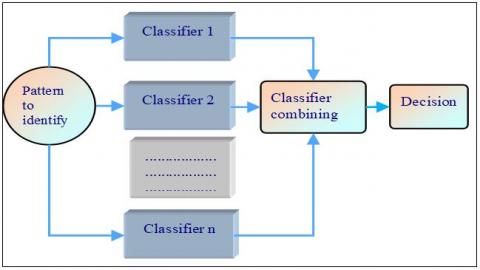
In our study, we have used the method of the parallel combination of classifiers which would submit the same characteristics to both classifiers and combine the results using a variety of methods, such as logistic regression and Borda Count, weighted sum... [9]. Each of the inducers is invoked independently, and their results are then combined by a combiner. The majority of combination architectures in the literature belong to this category. The problem with the parallel combination of classifiers may occur as follows [10]: given a set of K classifiers each it decides independently on a form to recognize, how to develop a single final response from the K results provided. This problem of the parallel combination requires first to remind what generally means "Classifier" as part of the combination then examine the criteria to be taken into account to categorize the different methods of combination presented in the literature (as shown in Figure 1).
Figure 1. The parallel combination of classifiers
2.2 Output types of combined classifiers
The way to categorize classifier combination is by the outputs of the classifiers used in the combination. Three types of classifier outputs are usually considered [11]:
Type I (abstract level): this is the lowest level since a classifier provides the least amount of information on this level. Classifier output is merely a single class label or an unordered set of candidate classes (Eq. (1)).
$ej\left( x \right)\text{ }=\left\{ Ci\text{ }/\text{ }i\text{ }<=\text{ }m \right\}$ (1)
Type II (rank level): classifier output on the rank level is an ordered sequence of candidate classes, the so-called n-best list. The candidate class at the first position is the most likely class, while the class positioned at the end of the list is the most unlikely. Note that there are no confidence values attached to the class labels on the rank level. Only their position in the n-best list indicates their relative likelihood (Eq. (2)).
$ej\left( x \right)\text{ }=\left[ rj1,\text{ }rj2,\text{ }\ldots ,\text{ }rjm \right] (2)
where, rj, i is the rank assigned to a class (i) by the classifier (j).
Type III (measurement level): In addition to the ordered n-best lists of candidate classes on the rank level, classifier output on the measurement level has confidence values assigned to each entry of the n-best list. These confidences, or scores, can be arbitrary real numbers, depending on the classification architecture used. The measurement level contains, therefore, most information among all three output levels (Eq. (3)).
$ej\left( x \right)\text{ }=\left[ rj1,\text{ }rj2,\text{ }\ldots ,\text{ }rjm \right]$ (3)
where, Mji is the measure assigned to a class (i) by the classifier (j).
To overcome the limitations of the high complexity and the no scale with the size of the very large datasets of the individual classifier, we have developed in this paper ISVM-LEARN++: A combination of two incremental supervised algorithms: incremental SVM and Learn++ (incremental neural network).
The proposed ISVM-LEARN++ consists of four subsystems (as shown in figure 2), which are batch datasets; Incremental SVM of [8]; the Learn ++ of [4] and the ISVM-Learn ++ Combination Module. The two main reasons for combining classifiers are efficiency and accuracy [12].
This section introduces a framework for using dynamic weighting ensembles to effectively learn new batches of data appearing over time without the need for retraining. There are two phases in the proposed algorithm (see Figure 2).
The first phase is to train an ensemble of incremental classifiers based on each batch of the input data when a new batch of data becomes available, a new ensemble of basic classifiers is built solely on it so that the new information can be effectively extracted, without interfering with existing classifiers. Another advantage is that the training process has much better flexibility than the retraining strategy. The second phase is to combine the outputs from individual incremental classifiers; the weighted sum method is used to combine all the incremental classifiers.
Figure 2. The proposed architecture of ISVM-LEARN++
The main idea behind this method is to build an extra model upon each basic classifier based on its training results (whether a training sample is classified correctly or not). By doing so, this new model is able to estimate the accuracy or the competency of the classifier for each new sample.
Special features of our combination are:
In what follows, we describe in details the main subsystems of ISVM-LEARN++:
3.1 Classifiers choice
The choice of classifiers is a difficult task; it has pushed researchers to develop methods to help designers. The simplest and most used method belongs to the static selection (Overproduce and choose), which consists of generating different classifiers based on the methods of creating sets and then choosing the group of classifiers whose output can then be combined and the combination produces the best result. In a simpler way, the main idea of this method is to produce a large initial set of candidate classifiers, then select a subset that is considered most valuable to achieve optimal performance.
To do this, the process follows two cycles:
We built a set of classifiers: Learn ++, ISVM from Cauwenberghs and Poggio, SVM from Diehl and Cauwenberghs [13] and ITI (Incremental Tree Inducer) of Utgoff [14]. We tested this dataset before doing the combination on a chosen database and we found that incremental SVM Cauwenberghs and Poggio and Learn ++ give optimal performance over leftovers.
3.2 Incremental SVM learning of Cauwenberghs and Poggio
Cauwenberghs and Poggio [8] propose an on-line, recursive algorithm for learning an SVM. Initially, a new example is added to the training database. If this is rated by the SVM then no change will be made. Otherwise, an update is necessary by making modifications to the Lagrange multipliers while respecting the conditions of Karush Kuhn Tucker (KKT).
The training dataset is partitioned into three groups:
After having initialized the optimal hyperplane of the model at the beginning of the classification, the objective is to adapt, sequentially, this hyperplane according to the evolution of the model over the sequence. When updating the decision boundary, examples from these three groups (D, S, U) may change state (when adding new data). A LOO (Leave One Out) decremental learning procedure is executed to delete old data. The basic idea is to adapt to the decision boundary to adding the new example to the solution and then removing those too old keeping the conditions of KKT satisfied.
Algorithm:
Let F be the training dataset and H (x) the separating function is reduced to a linear combination of the kernel function on the training data. The Lagrange multipliers are obtained by minimizing the convex quadratic objective function under the constraints (Eq. (4)):
Minimizes
$\mathrm { w } = \frac { 1 } { 2 } \sum _ { i = 1 } ^ { n } \sum \mathrm { j } = 1 ^ { \mathrm { n } } \alpha _ { \mathrm { i } } \alpha _ { \mathrm { j } } \mathrm { k } \left( \mathrm { x } _ { \mathrm { i } } , \mathrm { x } _ { \mathrm { j } } \right) - \sum _ { \mathrm { i } = 1 } ^ { \mathrm { n } } \alpha _ { \mathrm { i } } + \mathrm { b } \sum _ { \mathrm { i } = 1 } ^ { \mathrm { n } } \mathrm { y } _ { \mathrm { i } } \alpha _ { \mathrm { i } }$ (4)
1st order conditions on the W gradient lead to the following KKT conditions
$g i = j k ( x i , x j ) + b = H ( x i )$ (5)
$H ( x i ) > 0 \quad \alpha i = 0$
$H ( x i ) = 0$
$0 < \alpha i < C ; \frac { \partial w } { \partial b } = \sum _ { j = 1 } ^ { s } \alpha j - 1 = 0$ (6)
$H ( x i ) < 0$ if $\alpha = C$ {C is the regularization parameter}
3.2.1 Incremental learning procedure
When the new example xc is added to the set of support points S, the decision function is adapted and updated iteratively, that is to say, that its parameters αj, b are updated and recalculated so that iterative and incremental. At each iteration, gc = Hc (xc) is recalculated until gc = Hc (xc) = 0 while keeping the KKT conditions satisfied. We must then define the incrementation steps Δgi (with i = 1, ..., d), Δαi (with i = 1, ..., s) and Δb. To use the Lagrangian in solving constrained optimization equations, the Jacobian matrix Q is used.
The incremental learning procedure summary of a new example xc:
|
Initialization αc to zero If gc> 0, add xc to D. update G (GS + $1 \leftarrow \mathrm { G } _ { \mathrm { C } } ^ { \mathrm { S } }$ ), End. If gc = 0, add xc to S, update the parameters αj, b, R and G, End. If gc <0, add xc to U, as long as gc <0 do αc = αc + Δb Calculate β Calculate Δb, then b = b + βb For each $\mathrm { xj } \in \mathrm { S }$, calculate Δαj, then αj = αj + Δαj For each $\mathrm { xj } \in \mathrm { D }$, calculate Δgi, then gi = gi + Δgi Check if an example of the support is found inside the hyperplane ($\alpha j \leq 0$). If yes, Remove it from S and add it to D, and update all the parameters. Repeat until gc = 0 |
3.2.2 Decremental learning procedure
Incremental learning is the way to learn little by little, as data arrive. In contrast, the decremental learning is unlearning, to gradually forget knowledge from the oldest learning data [15]. The procedure for deleting old data is complementary to the procedure of adding new data. When an example xr is removed from S, gr will be removed from G and z (set of parameters {b, αr}) will be updated decremental and the decision function Hk will be adjusted up to that xr is outside (αr≤0). The matrix R is updated by removing from the matrix Q the column r + 1 and the line r + 1 (corresponding xr to which was removed). When an example xr is removed from D, the only G is updated by removing it gr.
Decremental learning procedure summary of an old example xr:
|
If gr = 0, remove xr from F, and remove gr from G (G ← G-gr), End. If gr = 0, remove xr from S, and therefore from F. As long as αr> 0 do αr = αr + Δα Calculate Δb, then b = b + Δb For each $\mathrm { xj } \in \mathrm { S }$, Calculate Δαj, then αj = αj-Δαj For each $\mathrm { xj } \in \mathrm { F }$, calculate Δg i, then gi = gi - Δgi Check if an inside example $\mathrm { xi } \in \mathrm { D }$ is outside the deciding boundary (Gi≤0). If yes, discontinue the deletion procedure, and apply the procedure add-on xi, so that the procedure of forgetting can be restored until αr = 0. |
3.3 Learn++
Learn ++ [4-16] is an incremental learning algorithm of a neural network inspired by the AdaBoost algorithm [17]. It is based on the principle of a combination of weak classifiers to make a decision. The system will train several classifiers on several subsets of the learning set. The difficulties of this algorithm lie in the creation of the training subsets and the combination of these classifiers. The idea of Learn ++ is to modify the distribution of the elements in the training subset in order to reinforce the presence of the most difficult elements to classify according to the errors of the weak classifier generated. This procedure is then repeated with a different set of data from the same learning base and new classifiers are generated. The output will be the combination of the outputs of the classifiers using the majority vote. The weak classifiers are classifiers that provide a rough estimate of a decision rule because they must be very fast to generate.
|
The pseudo-code of Learn++ |
|
Input: For each database drawn from Dk {k=1,2,……..,k} Sequence of m training examples S=[(x1,y1),(x2,y2),……(xm,ym)] Weak learning algorithm WeakLearn Integer Tk, specifying the number of iterations. Do for k=1,2,…... k Initialize w1(i) = D(i) = 1/m ∀i unless where is prior knowledge to select otherwise. Do for t=1,2,….Tk :
If ɛ t> ½ then t = t −1, discard ht and go to step 2. Otherwise, compute normalized error as βt = ɛt / (1- ɛt).
If Et > 1/2 then t=t-1 discard Ht and go to step 2. Set $\beta _ { t } = \frac { E _ { t } } { 1 - E _ { t } }$ (normalized composite error), and update the weights of the instances: $w _ { t + 1 } ( i ) = w _ { t } ( i ) \times \left\{ B _ { t } , s i H _ { t } \left( x _ { i } \right) = y _ { i } \right\}$
$H _ { \text {final} } = \arg \max _ { y \in Y } \sum _ { k = 1 } ^ { K } \sum _ { t: H _ { t } ( x ) = y } \log | \left( 1 / \beta _ { t } \right)$ |
3.4 Combination module
The combination choice module or the decision function plays a very important role in the design of a Multi Classifiers System (MCS) [18-19]. The output of the MCS reflects the decision of the whole set using, for example, the Bayesian method, the weighted sum.... The combination mechanism will be more effective when the classifiers exhibit different behaviors.
The combination method we have adopted for our system is the weighted sum method which is defined in the previous chapter as a generalization of the Borda Count method [20] in which the ranks assigned by a classifier are weighted by a coefficient indicating the importance given to this one. It consists in weighting the sum of the ranks according to the credibility or the confidence granted to the classifier.
In our system, each of the two classifiers presented above gives a result xki corresponding to the output class (k = 1..2) corresponds to the number of the classifier,
i correspond to the number of the class for each database.
To apply the weighted sum, we used weighting to represent the notion of trust given to the classifier. This degree of confidence is known a priori in the training phase and in the test phase, for that we consider that:
Let x1i, x2i be the outputs associated with class i for each classifier.
Let dc1, dc2, dc3 be the degrees of confidence of each of the classifiers determined by the recognition rate during the test phase.
The weighted sum method is then applied (see Eq. (7)):
$X i = \frac { X 1 i { \times } d c 1 + X 2 i { \times } d c 2 } { d c 1 + d c 2 }$ (7)
This formula is applied for all outputs obtained by each classifier and for all database packages.
In order to evaluate the performance of ISVM-LEARN++ algorithm, experiments are conducted on three data sets from UCI repository (refer Table 1): Haberman's Survival, Blood Transfusion Service Center and Ionosphere.
Table 1. Description of UCI databases
|
Dataset |
N°. of instances |
N°. of attributes |
Attributes type |
Missing values |
|
Haberman's Survival |
306 |
3 |
Integer |
No |
|
Blood Transfusion Service Center |
748 |
5 |
Real |
No |
|
Ionosphère |
351 |
34 |
Integer and real |
No |
Recognition rate (see Eq. (8)) is what we usually mean when we use the term accuracy. It is the ratio of a number of correct predictions to the total number of input samples.
Re cognition rate $= \frac { \text { Number of correct predictions } } { \text { Total nmber of predictions made } }$ (8)
Classification error rate (see Eq. (9))
Success: instance’s class is predicted correctly (True Positives (TP) / Negatives (TN))
Error: instance’s class is predicted incorrectly (False Positives (FP) /Negatives (FN))
Classification error rate (Eq. (9)): the proportion of instances misclassified over the whole set of instances
Errorrate$= \frac { F P + F N } { T P + T N + F P + F N }$ (9)
We have divided each ionosphere database into batches and we have introduced to each classifier a batch … The database is divided into 2 batches for training and the 3rd for testing. We choose sigma = 0.25 fixed, the parameter C = 10:
Table 2 summarizes the results obtained by running incremental SVM and Learn ++ on the three databases.
For the test phase, we took 1/3 of each database; the recognition rates of each class with respect to each classifier after the combination are mentioned in Table 3.
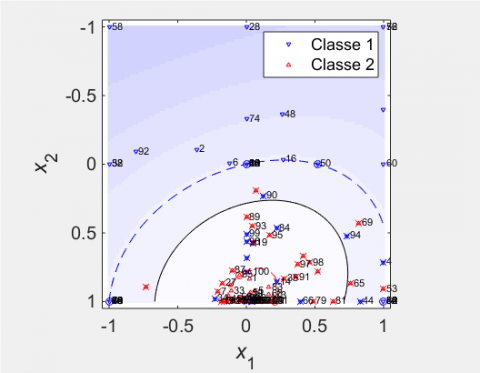
Figure 3. Classification by incremental SVM training dataset 1, C = 10, Sigma = 0:25, TB1 = 1-117, Vectors Errors = 42, recognition rate = 58 %
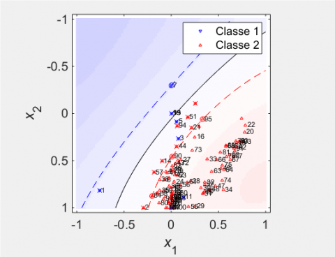
Figure 4. Classification by incremental SVM training dataset 2, C = 10, Sigma = 0.25, TB2 = 118- 234, Vectors Errors = 41, recognition rate = 59 %
Figure 5. Classification by incremental SVM testing dataset C = 10, Sigma = 0:25, TB = 235- 351, Vectors Errors = 17, recognition rate = 68 %
Table 2. The recognition rate of training datasets
|
Dataset |
Incremental SVM |
Learn++ |
|||||
|
C (regularization parameter) |
Sigma |
Vectors errors |
Recognition rate (%) |
T (N° of iterations) |
Error rate (%) |
Recognition rate (%) |
|
|
ionosphere_training1 (1_117) |
10 |
0.25 |
42 |
58 |
3 |
28.53 |
71.47 |
|
ionosphere _ training2 (118_234) |
10 |
0.25 |
41 |
59 |
3 |
16.38 |
83.62 |
|
Transfusion‑ training1 (1_88) |
10 |
0.25 |
32 |
68 |
3 |
50.20
|
49.80 |
|
Transfusion‑ training2 (89_176) |
10 |
0.25 |
20 |
80 |
3 |
38.43
|
61.57 |
|
Haberman‑ training1 (1_102) |
10 |
0.25 |
20 |
80 |
3 |
21.67 |
78.33 |
|
Haberman_ training2 (103_204) |
10 |
0.25 |
13 |
87 |
3 |
14.67 |
85.33 |
|
Data set |
Incremental SVM |
Learn++ |
|||||
|
C (regularization parameter) |
Sigma |
Vectors errors |
Rate recognition (%) |
T (N° of iterations) |
Error rate (%) |
Recognition rate (%) |
|
|
ionosphere _test (235_351) |
10 |
0.25 |
17 |
83 |
3 |
9.32 |
90.68 |
|
Transfusion_test (177_264) |
10 |
0.25 |
22 |
78 |
3 |
26.67 |
73.33 |
|
Haberman_test (205_306) |
10 |
0.25 |
20 |
80 |
3 |
43.33 |
56.67 |
|
Data set |
Incremental SVM |
Learn++ |
Combination (X) |
||||||
|
Vectors errors |
Recognition rate |
Class 1 |
Class 2 |
Rate error |
Recognition rate |
Class 1 |
Class 2 |
||
|
Ionosphere test 235_351 |
17 |
0.83 |
44 |
56 |
0.0932 |
0.9068 |
23 |
94 |
0.93 |
|
Transfusion test 177_264 |
22 |
0.78 |
66 |
0 |
0.2667 |
0.73 |
17 |
71 |
0.87
|
|
Haberman test 205_306 |
20 |
0.80 |
1 |
81 |
0.4333 |
0.57 |
20 |
82 |
0.88 |
We remark that the number of error vectors is large in Figure 3 = 42, as well as the margin increases, so the performance decreases = 58 %, even Figure 4, the performance is almost equal to 59 %, it is the same for the 1st training batch. If we look at the third case (Figure 5), we find that the number of error vectors is 17, the margin is small, the performance is not better (68 %). So the best case is the third, we observe the number of errors equal to 32 % that is to say we agreed to have misclassified points.
Combination results:
After having seen the results of the two individual classifiers, we combined the two in parallel using a weighted sum combination, we took the degrees of confidence of each of the classifiers the recognition rate during the test phase, applying the formula (7) on the Ionosphere database, and we obtain the following results:
Let x1i, x2i be the outputs associated with class i for each classifier that take the values given in Table 4.
Let dc1, dc2, dc3 be the confidence levels of each of the following values: 0.83-0.78-0.80-0.9068-0.70-0.57:
The weighted sum method is then applied:
$\mathrm { X } _ { \mathrm { i } } = \frac { \left( \mathrm { X } _ { 1 \mathrm { i } } \times \mathrm { d } \mathrm { c } 1 + \mathrm { X } _ { 2 \mathrm { i } } \times \mathrm { d } \mathrm { c } 2 \right) } { ( \mathrm { d } c 1 + \mathrm { d } \mathrm { c } 2 ) }$ (10)
We calculated the outputs for each classifier and for each database; we obtained the following results (see Table 4):
Weighted Sum1 = ((0.83 * (44/117) + 0.83 * (56/117)) + ((0.9068 * (23/117) + 0.9068 * (94/117)))) / ((0.83 + 0.9068)) = 0.93
The performance obtained after combining the two classifiers on the 1st database is: 93% and 7% rejection.
Weighted Sum2 = ((0.78 * (66/88) + 0.78 * (0/88)) + ((0.73 * (17/88) + 0.73 * (71/88)))) / ((0.78 + 0.73)) = 0.87
The performance obtained after the combination of the two classifiers on the 2nd database is: 87% and 13% rejection.
Weighted Sum3 = ((0.8 * (1/102) + 0.8 * (81/102)) + ((0.57 * (20/102) + 0.57 * (82/102)))) / ((0.8 + 0.57)) = 0.88
The performance obtained after the combination of the two classifiers on the 3rd database is: 88% and 12% rejection.
According to our proposed architecture (Fig.2), the final decision is the combination of the classifier combinations, so we will apply the weighted sum on the previous results (X of Table 5).
Table 5. Final combination results
|
Data set |
Classifiers combination (ISVM-Learn++) |
||
|
X |
Class1 |
Class2 |
|
|
Ionosphere test 235_351 |
0.93 |
67 |
150 |
|
Transfusion test 177_264 |
0.87 |
83 |
71 |
|
Haberman test 205_306 |
0.88 |
21 |
163 |
|
Final combination results |
0.98 |
||
Final weighted sum =$\left(\frac{ { \left( 0.93 * \left( \frac { 67 } { 217 } \right) + 0.93 * \left( \frac { 150 } { 217 } \right) \right) + \left( 0.87 * \left( \frac { 83 } { 154 } \right) + 0.87 * \left( \frac { 71 } { 154 } \right) \right) } \\ { + \left( 0.88 * \left( \frac { 21 } { 184 } \right) + 0.88 * \left( \frac { 163 } { 134 } \right) \right) } }{ { ( 0.93 + 0.87 + 0.88 ) } } \right) = 0.98$
The performance obtained after the combination of the two classifiers on the 3rd database is 98 % and 2 % rejection.
The performance results of individual classifiers and multi-classifiers are summarized in Table 6.
Table 6. Final combination performance results
|
Classifiers |
Recognition rate(%) |
|
Incremental SVM and Learn++ (First BDD) |
93 |
|
Incremental SVM and Learn++ (Second BDD) |
87 |
|
Incremental SVM andt Learn++ (ThirdBDD) |
88 |
|
ISVM-Learn++ |
98 |
The recognition rate has been increased with the combination of 5 % compared to the best classifier and by 11 % compared to the average of the three combinations, it can be deduced that with the use of the combination of classifiers we benefit from the powers individual classifiers, each in his specialty space for a higher recognition rate.
The ultimate goal of our work is the combination of incremental classifiers ISVM-Learn ++ involving several incremental classifiers to take advantage of their performance and increase the recognition rate, so we tried to vary the classifiers by choosing them of a different nature. For this purpose, a committee of two incremental classifiers was studied, namely the incremental SVM of Cauwenberghs et al. and Learn ++.
To evaluate our classifiers and their combination on diversified data, three databases were used from UCI (University California Irvine) repository: Ionosphere, Haberman's Survival and Blood Transfusion Service Center repository.
Each of the two incremental classifiers was developed separately with part of the training dataset, and their respective parameters were therefore released. We then tested each of them on the same basis of validation, then we applied the combination, the 98 % rate of good recognition reinforces the fact that the combination gives better performance than any other classifier taken individually.
In the future, we can analyze the complexity of the proposed algorithm for evolving machine learning and we can investigate several other combinations methods of different incremental classifiers, for comparison purposes. For example, it is possible to integrate an incremental classifier based on the ITI decision trees, for example, in the combination and try to benefit from the ITI power shown in recent work. We also plan to compare between the combination of ILbyCC classifiers and our proposed ISVM-Learn ++ classifier.
The authors are grateful to the anonymous referees for their very constructive remarks and suggestions.
[1] Almaksour, A. (2011). Incremental learning of evolving fuzzy inference systems: Application to handwritten gesture recognition. Ph.D. thesis, INSA, Rennes.
[2] Chefrour, A. (2019). Incremental supervised learning: algorithms and applications in pattern recognition. Evolutionary Intelligence, 12(2): 97-112. https://doi.org/10.1007/s12065-019-00203-y
[3] Ianakie, K., Govindaraju, V. (2002). Architecture for classifier combination using entropy measures. In International Workshop on Multiple Classifier Systems, pp. 340-350. https://doi.org/10.1007/3-540-45014-9_33
[4] Polikar, R., Upda, L., Upda, S.S., Honavar, V. (2001). Learn++: An incremental learning algorithm for supervised neural networks. IEEE Transactions on Systems, Man, and Cybernetics, Part C (Applications and Reviews), 31(4): 497-508. https://doi.org/10.1109/5326.983933
[5] Muhlbaier, M., Topalis, A., Polikar, R. (2004). Learn++. MT: A new approach to incremental learning. In International Workshop on Multiple Classifier Systems Springer, Berlin, Heidelberg, pp. 52-61. https://doi.org/10.1007/978-3-540-25966-4_5
[6] Muhlbaier, M.D., Topalis, A., Polikar, R. (2009). Learn++. NC: Combining ensemble of classifiers with dynamically weighted consult-and-vote for efficient incremental learning of new classes. IEEE Transactions on Neural Networks, 20(1): 52-168. https://doi.org/10.1109/TNN.2008.2008326
[7] Wen, Y.M., Lu, B.L. (2007). Incremental learning of support vector machines by classifier combining. In Pacific-Asia Conference on Knowledge Discovery and Data Mining Springer, Berlin, Heidelberg, pp. 904-911. https://doi.org/10.1007/978-3-540-71701-0_101
[8] Cauwenberghs, G., Poggio, T. (2001). Incremental and decremental support vector machine learning. In Advances in Neural Information Processing Systems, pp. 409-415.
[9] Bahler, D., Navarro, L. (2000). Methods for combining heterogeneous sets of classifiers. In 17th Natl. Conf. on Artificial Intelligence (AAAI), Workshop on New Research Problems for Machine Learning.
[10] Ponti Jr., M.P. (2011). Combining classifiers: from the creation of ensembles to the decision fusion. In 2011 24th SIBGRAPI Conference on Graphics, Patterns, and Images Tutorials, pp. 1-10. https://doi.org/10.1109/SIBGRAPI-T.2011.9
[11] Tulyakov, S., Jaeger, S., Govindaraju, V., Doermann, D. (2008). Review of classifier combination methods. In Machine Learning in Document Analysis and Recognition Springer, Berlin, Heidelberg, pp. 361-386. https://doi.org/10.1007/978-3-540-76280-5_14
[12] Kittler, J., Hatef, M., Duin, R.P., Matas, J. (1998). On combining classifiers. IEEE Transactions on Pattern Analysis and Machine Intelligence, 20(3): 226-239. https://doi.org/10.1109/34.667881
[13] Diehl, C.P., Cauwenberghs, G. (2003). SVM incremental learning, adaptation and optimization. In Neural Networks, Proceedings of the International Joint Conference on IEEE, pp. 2685-2690. https://doi.org/10.1109/IJCNN.2003.1223991
[14] Utgoff, P.E. (1994). An improved algorithm for incremental induction of decision trees. In Proceeding of the 11th International Conference on Machine Learning, New Brunswick, NJ, Morgan Kauffmqan, pp. 318-325. https://doi.org/10.1016/B978-1-55860-335-6.50046-5
[15] Bouillon, M., Anquetil, E., Almaksour, A. (2013). Decremental learning of evolving fuzzy inference systems: application to handwritten gesture recognition. In International Workshop on Machine Learning and Data Mining in Pattern Recognition Springer, Berlin, Heidelberg, pp. 115-129. https://doi.org/10.1007/978-3-642-39712-7_9
[16] Patel, A.J., Patel, J.S. (2013). Ensemble systems and incremental learning. In 2013 International Conference on Intelligent Systems and Signal Processing (ISSP), pp. 365-368. https://doi.org/10.1109/ISSP.2013.6526936
[17] Zhao, Q.L., Jiang, Y.H., Xu, M. (2010). Incremental learning by heterogeneous bagging ensemble. In International Conference on Advanced Data Mining and Applications, pp. 1-12. https://doi.org/10.1007/978-3-642-17313-4_1
[18] Ranawana, R., Palade, V. (2006). Multi-classifier systems: Review and a roadmap for developers. International Journal of Hybrid Intelligent Systems, 3(1): 35-61. https://doi.org/10.3233/HIS-2006-3104
[19] Dahmouni, A., Aharrane, N., El Moutaouakil, K., Satori, K. (2017). Multi-classifiers face recognition system using LBPP face representation. International journal of Innovative Computing Information and Control, 13(5): 1721-1733.
[20] Koffi, C. (2015). Exploring a generalized partial Borda count voting system. Senior Projects Spring 2015.
[21] Abbas, E.I., Safi, M.E., Rijab, K.S. (2017). Face recognition rate using different classifier methods based on PCA. In 2017 International Conference on Current Research in Computer Science and Information Technology (ICCIT), pp. 37-40. https://doi.org/10.1109/CRCSIT.2017.7965559