Sanjay Agrawal | Rutuparna Panda* | Swati Kumari | Lingraj Dora | Ajith Abraham
OPEN ACCESS
The limited depth of field in optical lenses and camera leads to output images having non-uniform focus. Fusing the focussed regions from many images of the identical scene results in an output image with uniform focus. Generally, the methods suggested for image fusion (IF) suffers from computational complexity. In this context, we suggest a new hybrid multifocus IF model using a single optimum Gabor filter. Another important contribution of this paper is that the Gabor filter is capable of distinguishing the clear and the blurry pixels. The key concept is to decompose inputs into blocks. Each of the blocks/patches is convolved with the single optimum Gabor filter for extracting the Gabor energy feature vector. A new patch is created for fusion based on the Gabor energy feature value of each pixel in the patch. The parameters of the single Gabor filter are optimized using a relatively new optimization technique termed squirrel search algorithm (SSA). The application of optimal Gabor filter to the multifocus image fusion problem is new. The suggested technique is tested with standard images having focus on distinct objects. The outcomes reveal that the suggested technique provides improved performance, it outperforms state-of-the-art classic fusion approaches in both objective and subjective assessments.
Gabor energy feature, Gabor filter bank, multifocus image fusion, optimum Gabor filter, squirrel search algorithm
Image fusion has grown as a key topic of investigation in recent times. It combines the source images acquired from various sources into a sole output image. Compared to the individual source images, the output image is better suited for human viewing or image processing functions. Many IF applications are reported in the literature. The popular ones being multi-spectral, multi-modal, multi-sensor and multifocus IF. This work addresses the multifocus IF problem. Even though the sensor technology has improved significantly, it is not possible for optical lenses or camera having finite depth of field to acquire an image having all the regions in focus. So, a single image acquired cannot give us all the required information. Further, analysing similar images individually leads to time consumption and complexity. To solve such problems, multifocus IF merges relevant info from two or more images of the identical scene to generate the output. The output will include all the required info [1-2]. Now multifocus IF is applied in numerous applications for instance, medical imaging [3], optical microscopy [4-5], surveillance and many other fields [6-7].
IF is usually done at 03 levels – pixel, feature and decision level. The pixel based IF techniques consider directly the pixels of the input images. The intensities of the pixels are processed for defining the fusion task. Usually, it is less complex and simple to implement. However, these schemes bring into blurring effects and does not handle cases of misregistration well. The feature level IF techniques extract features such as shape, size, and contrast before the fusion process. The continuous regions in the input images are identified using suitable segmentation techniques. Then a region level fusion scheme is followed to get the output. The decision based IF methods take the inputs from the feature level techniques and use the image descriptors for fusion [8].
This paper uses both the pixel and the feature level fusion technique. In another context, IF is implemented in spatial domain and transform domain. In the former case, the focused pixels are chosen directly from the source images and the output is obtained by following suitable fusion rules. For instance, the averaging of the pixel intensities from both the source images to get the output is one of the simplest methods in fusion. However, there are lots of drawbacks – i) the correlation between the neighbouring pixels is not taken into account and ii) it reduces the contrast. In transform domain, the source images are converted using suitable transform functions. The fusion is implemented in the transform domain [9-10]. Then inverse transformation function is utilized to get the output. This paper follows the spatial domain fusion scheme.
Numerous multifocus IF techniques are reported in the literature. A comprehensive review on region based IF techniques is carried out in [11]. Phamila and Amutha [12] suggested use of discrete cosine transform (DCT) for multifocus fusion in sensor networks. The authors chose higher valued AC coefficients in the transformed block for fusion. They used a number of metrics for comparison. They concluded that if the output is stored as JPEG, then the proposed method is efficient. Wan et al. [13] suggested robust principal component analysis (RPCA) for multifocus IF. The authors compared their results with wavelet based fusion methods. They concluded that their method performs better but having low computational efficiency. Liu et al. [14] proposed a method utilizing dense scale invariant feature transform (SIFT) for multifocus IF. The authors stated that their technique is superior to other methods in objective evaluation and visual assessment. However, the memory requirements for the method is high. Wu et al. [15] utilized Hidden Markov Model (HMM) for the fusion. The authors divided the input images into overlapping patches. Each patch’s clarity and fidelity are used to model the fused image. The suggested method gives improved visual perception in comparison to multiscale transform method. It is suitable for misregistered images.
Singh and Khare [16] used the multi-resolution principle for IF. They applied Daubechies Complex Wavelet Transform (DCWT) and used maximum selection rule to fuse the wavelet coefficients. The authors claimed that their approach is superior to the other wavelet based methods. Bai et al. [17] presented a quad tree based fusion scheme utilizing weighted focus measure. The authors used sum of the weighted modified Laplacian to determine the weight measure to detect the focussed block. The suggested method gives speed advantage in comparison to other transform based techniques. Yin et al. [18] suggested a fusion procedure utilizing compressive sensing. The authors used non-subsampled contourlet transform to divide the source images. The authors claimed to achieve great details and saliency characteristics in the output. Li et al. [19] utilized decomposition utilizing sparse matrix and morphological filtering for multifocus IF. The authors stated that their method performs better than RPCA. However, their method does not preserve the source image pixel values. Recently, many multi focus IF schemes are proposed utilizing content adaptive blurring [20], convolution neural network [21], different wavelet transforms [22], sparse representation [23], pulse coupled neural network [24] and adaptive principal component analysis [25].
The above study outlines a number of multifocus IF techniques. The emphasis is on better visual perception and performance metrics. This has motivated us to suggest a new hybrid fusion technique utilizing a single optimum Gabor filter for improved performance. The Gabor filter parameters are optimized using SSA [26]. The input images are decomposed into patches. The Gabor energy feature is obtained by convolving each input image patch with the single optimum Gabor filter. A new patch is created by comparing each patch from both the input images based on maximum Gabor energy. The output is formed by using the new patches formed. The suggested scheme is compared with many multi-source IF techniques: filter-subtract-decimate (FSD) pyramid IF procedure [27], DWT IF procedure [28], contrast pyramid IF technique [29], shift-invariant DWT (SIDWT) IF method [30] and the spatial frequency (SF) fusion method [31]. Various performance metrics are computed for comparison.
It is perceived that the suggested technique gives improved performance in comparison to the state-of-the-art techniques. The contributions of this work are: 1) Conventional filter bank approach is substituted by a single optimal Gabor filter for the problem on hand. This scheme allows optimal selection of Gabor parameters, optimal feature extraction and reduce the high dimensionality problem, 2) The advantages of pixel and feature based fusion approaches are merged to get the output. To the best of our knowledge, the application of a single optimum Gabor filter to multifocus image fusion problem is not reported in the literature.
The remaining manuscript is structured as: Section 2 briefly explains the optimum Gabor filter concept. Section 3 explains the suggested procedure. Results and discussions are presented in Section 4. Lastly, the conclusion is presented in Section 5.
2.1 Gabor filter bank
A number of researchers have explored Gabor filter for feature extraction task. It is extensively utilized in several applications like pattern recognition, texture classification, etc. Gabor filters are orientation-sensitive filters used in image processing, mainly for edge and texture analysis. The kernels of the filter resemble the 2D receptive field profile of human cortical cells. Therefore, they have optimum localization features in both spatial as well as frequency domain analysis. The Gabor filter is represented as a complex exponential function modified by a Gaussian term in the spatial domain. It is expressed as:
$\varphi ( x , y , \omega , \theta ) = \frac { 1 } { 2 \pi \sigma ^ { 2 } } e ^ { - \left( \frac { x ^ { \prime 2 } + y ^ { \prime 2 } } { 2 \sigma ^ { 2 } } \right) \left[ e ^ { i \omega x ^ { \prime } } - e ^ { - \frac { \omega ^ { 2 } \sigma ^ { 2 } } { 2 } } \right] }$ (1)
where, $x ^ { \prime } = x \cos \theta + y \sin \theta , \quad y ^ { \prime } = - x \sin \theta + y \cos \theta$.
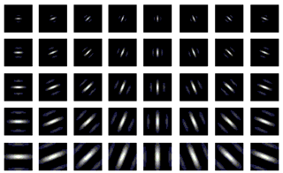
Here (x,y) represents the pixel location in spatial domain, ω is the radial frequency, θ symbolizes the direction of the filter, σ signifies the standard deviation of the Gaussian function. A Gabor filter bank is constructed with different frequencies and directions. The real part of a sample Gabor filter bank with 05 frequencies and 08 directions is presented in Figure 1. The rows in Figure 1 represents variations in frequencies ωm and the columns represent variations in orientations θn.
Figure 1. Example Gabor filter bank
The following simplified two-dimensional (2D) Gabor function is utilized to form the filter bank.
$g _ { \lambda , \theta , \varphi , \sigma , \gamma } = \exp \left( - \frac { x ^ { \prime 2 } + \gamma ^ { 2 } y ^ { \prime 2 } } { 2 \sigma ^ { 2 } } \right) \cos \left( 2 \pi \frac { x ^ { \prime } } { \lambda } + \varphi \right)$ (2)
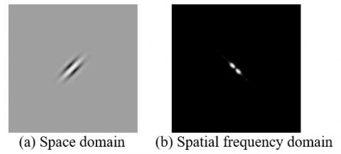
The λ parameter denotes wavelength and its reciprocal (1/λ) the spatial frequency. The factor γ denotes the spatial aspect ratio. The term (σ/λ) indicates the bandwidth of the filter. Note that θ represents the direction of the filter and its phase is represented by φ. The phase controls the symmetry of the filter. The range of values of all the parameters is given in literature [32-34]. An example 2D Gabor function in space and spatial frequency representation is displayed in Figure 2.
Figure 2. Example 2D Gabor function
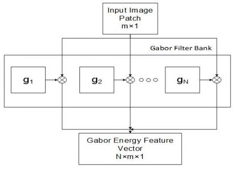
The Gabor filter response to an image i(x,y) is computed by convolving the filter defined in Eq. (2) with the image as $r ( u , v ) = i ( u , v ) \otimes g ( u , v )$. The symbol $\otimes$ indicates the convolution operation. The response is controlled by the parameters of the filter. Different parameters for a filter will yield discrete results for the identical input image. So a Gabor filter bank is designed using a group of Gabor filters with different phase, directions and spatial frequencies. This results in capturing most of the features of the image and deriving discriminatory and local features. The Gabor energy feature is computed after the filter responses from the phase pairs are merged. It is represented as,
$e _ { \lambda , \theta , \varphi , \sigma , \gamma } ( x , y ) = \sqrt { r _ { \lambda , \theta , \sigma , \gamma , \pi } ^ { 2 } ( x , y ) + r _ { \lambda , \theta , \sigma , \gamma , \pi / 2 } ^ { 2 } ( x , y ) }$ (3)
Here, $r _ { \lambda , \theta , \sigma , \gamma , \pi } ^ { 2 }$ and $r _ { \lambda , \theta , \sigma , \gamma , \pi / 2 } ^ { 2 }$ represents the response of the Gabor filters possessing phase pairs π and π/2 respectively [34]. A schematic block diagram for extraction of Gabor energy feature vector using a filter bank with N number of filters is shown in Figure 3.
Figure 3. Gabor energy feature vector extraction
The feature extraction task utilizing Gabor filter is accomplished in two different ways: 1) using filter bank approach as discussed above and 2) using optimal filter. However, the first scheme results in high dimension feature vectors and large response time. Moreover, for efficient feature extraction its performance heavily depends upon the filter parameters in the bank, which is usually done by trial and error.
To avoid these problems, use of a single optimal filter is a good alternative. The parameters of this filter are optimized using evolutionary algorithm to attain a particular task. Hence, a single optimal filter is sufficient enough for efficient feature extraction and thereby significantly reduces the response time [35]. Here, a novel approach for multifocus IF utilizing a single optimal Gabor filter is suggested. This is the first time a single optimum Gabor filter is investigated for the problem on hand. The choice of the parameters is suitable to maximize the performance of IF while reducing computational complexity and the exhaustive search. Here, a recently proposed optimization algorithm - SSA [26] is utilized to optimize the parameters of the Gabor filter. The objective function based on Gabor energy feature vector is utilized to get the optimum Gabor parameters. A block diagram for obtaining the optimum Gabor filter is shown in Figure 4.
Figure 4. Scheme for designing the optimum Gabor filter
2.2 Squirrel search algorithm
SSA, a recent nature inspired soft computing approach utilizing the foraging behaviours of the southern flying squirrel and their most effective way of movement called gliding. The squirrels have an inherent dynamic foraging scheme to optimally utilize the food resources. To model this technique, the following assumptions are used:
In this paper, n is taken 50. Nfs indicates the nutritious food resources, which is chosen as 4 (one hickory tree and three acorn nut trees), as suggested in Ref. [26]. The first position of every squirrel in the region of interest is expressed as:
$F S _ { i } = F S _ { L B } + R ( 0,1 ) \times \left( F S _ { U B } - F S _ { L B } \right)$ (4)
where, FSLB and FSUB are the lower and upper limits respectively of ith squirrel. Note that R(0, 1) is a uniformly distributed random numeral within [0, 1].
An objective function is used to calculate the fitness of flying squirrels at their respective position. These values denote the characteristics of nutrient resource explored by the individual i.e. optimum resource (hickory tree). It may be normal resource (acorn tree) or no resource (normal tree). This ultimately decides their chance of existence also. Any individual having minimum fitness is considered on hickory tree. The subsequent 03 best individuals are considered on acorn trees. Moreover, it is presumed that they are heading to the hickory tree. The rest of the individuals are assumed on normal trees. Furthermore, via random search, a few individuals are assumed to be heading to the hickory tree supposing that they consume their regular energy supplies.
The rest of the individuals will advance towards the acorn tree to fulfill their everyday nutrient needs. However, every time this foraging scheme is prone to predators. Thus, a predator presence probability (Pdp) is employed in the position update strategy. In every condition, the flying squirrel glides and seeks efficiently for the food resources, when the predator is absent. On the other hand, in the presence of predators, they take small random moves in the nearby area in search of food.
The foraging strategy is expressed as:
Case 1: If FSatdenotes the flying squirrel on the acorn trees can shift to the hickory tree, then their updated position is given as:
$F S _ { a t } ^ { g + 1 } = \left\{ \begin{array} { l l } { \left\{ F S _ { a t } ^ { g } + d _ { g } \times G _ { c } \times \left( F S _ { h t } ^ { g } - F S _ { a t } ^ { g } \right) r a n d 1 \geq P _ { d p } \right.} \\ { \text {random location} \quad \text { else } } \end{array} \right.$
where, dg is random gliding distance, rand1 is a random numeral within [0, 1]. FSht is the position of the squirrel that arrived at the hickory tree. Note that g represents the present iteration. The equilibrium between exploration and exploitation is accomplished utilizing the gliding constant Gc.
Case 2: If FSnt indicates the flying squirrel on the normal trees can shift to acorn trees then their new position is given as:
$F S _ { n t } ^ { g + 1 } = \left\{ \begin{array} { l } { \left\{ F S _ { n t } ^ { g } + d _ { g } \times G _ { c } \times \left( F S _ { a t } ^ { g } - F S _ { n t } ^ { g } \right) r a n d 2 \geq P _ { d p } \right.} \\ { \text {random location } \quad \text { else } } \end{array} \right.$
where, rand2 is another random numeral within [0,1].
Case 3: The squirrel on the normal tree with sufficient acorn nuts may likely to head towards the hickory nut tree. Their position is updated as:
$F S _ { n t } ^ { g + 1 } = \left\{ \begin{array} { l } { \left\{ F S _ { n t } ^ { g } + d _ { g } \times G _ { c } \times \left( F S _ { h t } ^ { g } - F S _ { n t } ^ { g } \right) r a n d 3 \geq P _ { d p } \right.} \\ { \text {random location} \quad \text { else } } \end{array} \right.$
where, rand3 is also a random numeral within [0,1].
This paper suggests a novel hybrid fusion scheme for multifocus images utilizing a single optimum Gabor filter. A schematic illustration of the proposed technique is displayed in Figure 5. The source images are read. Each image is partitioned into non-overlapping patches. In the beginning, the proposed method randomly initializes the parameters of the Gabor filter based on the constraints given below:
Table 1. Gabor filter parameters and constraints
|
Parameter |
Constraint |
|
Orientation, θ |
[0, π) |
|
Spatial frequency, f |
[0, 0.5] |
|
Aspect ratio, σ |
[0.23, 0.92] |
|
Bandwidth, B |
1.0 to 1.8 octaves |
$F = \sum \sum e ( x , y ) , F _ { o p t m a l } = \underset { P } { \operatorname { argmax } } \{ F \}$ (5)
Figure 5. Schematic illustration of the suggested technique
The evolutionary algorithm looks for the filter for which the objective function F is maximized.
A single optimum Gabor filter is designed from the above steps. Each patch is convolved with this filter to generate the Gabor energy feature vector. The two energy feature vectors obtained from both the input images at the same location are now considered. A new patch is created by comparing the Gabor energy values of the vectors. If the energy value of the first vector is larger, then that corresponding pixel from the first input image patch becomes a part of the new patch at the same location. Similarly, if the energy value of the second vector is larger, then that corresponding pixel from the second input image patch becomes a part of the new patch at the same location. In this way, a new patch is created for fusion of the images considering both the feature and pixel characteristics. This procedure is reiterated till all the patches are considered. Then the fused image is created after mapping the patches to their corresponding locations.
A pseudocode of the suggested technique is given below.
Step 1: Read the two input images (say size M×N) with
focus on different objects of the same scene.
Step 2: Divide each image into non overlapping patches, i.e.
patch size: w×w. Each patch is converted into a
column vector by lexicographic ordering, size: w2×1.
Step 3: Create a single optimum Gabor filter using Eq. (5).
Step 4: Convolve each image patch with the filter and compute
the Gabor energy feature vector resulting in w2×1
feature vector.
Step 5: Compare the Gabor energy feature vectors from both
the input image patches. If the energy $e _ { i _ { 1 } } > e _ { i _ { 2 } }$, then
the corresponding pixel at location i from the first
image becomes a part of the new patch. If $e _ { i _ { 1 } } < e _ { i _ { 2 } }$,
then the corresponding pixel at location i from the
second image becomes a part of the new patch.
Step 7: Repeat step 4 to step 6, until all the patches are
considered.
Step 8: Reconstruct the fused image after mapping the patches
to their corresponding positions.
The fusion rule is formed utilizing the maximum Gabor energy feature in each patch given as:
$I _ { f } ( u , v ) = \left\{ \begin{array} { l l } { I _ { A } ( u , v ) , } & { \text { If } e _ { A } ( u , v ) > e _ { B } ( u , v ) } \\ { I _ { B } ( u , v ) , } & { \text { If } e _ { A } ( u , v ) < e _ { B } ( u , v ) } \end{array} \right.$ (6)
where, If(u,v) represents the fused image patch, IA(u,v) represent the patch from input image A, IB(u,v) represents the patch from input image B, eA(u,v) represent the Gabor energy feature from patch A and eB(u,v) represent the Gabor energy feature from B.
So as to validate the efficacy of the suggested technique, four sets of multifocus image pairs from the grayscale dataset [36]: ‘clock’, ‘disk’, ‘pepsi’ and ‘lab’ are considered to experiment as displayed in Figure 6. Each set consists of two source images with different depth of focus.
Figure 6. Multifocus source images
For instance, Figure 6(a) contains two clock images with focus on right clock which is clearer, but the left clock is blurred. However, in Figure 6(b) the condition is swapped. A similar situation is observed in the other sets of images. The goal of this work is to produce a fused image with clearer objects with extended depth of focus. We have used five classic multi-focus IF procedures for a comparison using the same sets of input images. The pyramid fusion method and DWT uses Daubechies Spline DBSS (2,2) wavelets and SIDWT method uses Haar wavelets. The parameters are selected using unified rules of pyramid decomposition. The high frequency coefficients are chosen on ‘max’ value basis. The low frequency coefficients are selected on ‘average’ value basis. The number of layers for image transformation are taken four. A best block size of 8×8 is considered for the output in the SF method. The threshold for the SF algorithm is taken one.
The suggested procedure is realized in MATLAB using a core-i3 processor with 4GB RAM running under Windows 10 platform. We have used five objective performance measures: Mutual information (MI) [28], Average Gradient (AG) [28], Correlation Co-efficient (CC) [28], Distortion Degree (DD) [28], Petrovic metric (QAB/F) [29] for comparison. A brief discussion about the performance measures is presented below.
Mutual Information (MI): It indicates the information transferred from the input images to the output. The MI is computed between an input image Ii and the output If as:
$M I _ { i , f } = \sum _ { I_i , i _ { f } } h _ { i , f } \left( I _ { i } , I _ { f } \right) \log \frac { h _ { i , f } \left( I _ { i } , I _ { f } \right) } { h _ { i } \left( I _ { i } \right) h _ { f } \left( I _ { f } \right) }$ (7)
where, $h _ { i } \left( I _ { i } \right)$ and $h _ { f } \left( I _ { f } \right)$ signify the normalized histogram of the input and the output image respectively, $h _ { i , f } \left( I _ { i } , I _ { f } \right)$ implies the normalized joint histogram of the input and the output image. Now the total $M I$ computed as $M I _ { 1,2 , f } = M _ { 1 , f } + M _ { 2 , f }$ where $M _ { 1 , f }$ is the $M$ between the first input and the output. Likewise, $M _ { 2 , f }$ is the $M I$ between the second input and the output. A greater MI value is usually desired for good fusion performance.
Average Gradient (AG): This parameter measures an image’s clarity. A higher value of AG shows a clearer image, more image levels, and indicates a better quality of fusion. The AG is computed as:
$A G = \frac { 1 } { ( M - 1 ) ( N - 1 ) } \times$ $\sum _ { i = 1 } ^ { M - 1 - 1 } \sqrt { \frac { ( I ( i , j ) - I ( i + 1 , j ) ) ^ { 2 } + ( I ( i , j ) - I ( i , j + 1 ) ) ^ { 2 } } { 2 } }$ (8)
where, M, N represents the dimension of the image I. The term inside the parenthesis signifies the intensity value difference in the i and j directions.
Correlation Coefficient (CC): It computes the degree of linear coherence between the input images and the output. It is computed as:
$C C _ { f , i } = \frac { \sum _ { i , j } \left\{ I _ { f } ( i , j ) - \overline { I } _ { f } | \times \left[ I _ { i } ( i , j ) - \overline { I } _ { i } \right] \right\} } { \sqrt { \sum _ { i , j } \left[ I _ { f } ( i , j ) - \overline { I } _ { f } \right] ^ { 2 } \times \sum _ { i , j } \left[ I _ { i } ( i , j ) - \overline { I } _ { i } \right] ^ { 2 } } }$ (9)
where, $I _ { f } ( i , j )$ and $I _ { i } ( i , j )$ enotes the intensity values at location $( i , j )$ in the output and the input image respectively. $\overline { I } _ { f }$ and $\overline { I } _ { i }$ represent the corresponding mean grey values. A value of CC closer to one signifies a better fusion as the images will be more similar.
Distortion Degree (DD): The distortion degree signifies the image fidelity and is computed as
$D D _ { f , i } = \frac { 1 } { M \times N } \sum _ { i = 1 } ^ { M } \sum _ { j = 1 } ^ { N } \left| I _ { f } ( i , j ) - I _ { i } ( i , j ) \right|$ (10)
where, $I _ { f } ( i , j )$ and $I _ { i } ( i , j )$ represent the fused image and the input image respectively.
Petrovic Metric: It is also known as edge based similarity measure. It calculates the amount of edge info transmitted from inputs to the output. Mathematically, it is denoted as $Q ^ { A B / F }$ and is defined as [37-38]
$Q ^ { A B F } = \frac { \sum _ { i = 1 } ^ { M } \sum _ { j = 1 } ^ { N } \left[ Q _ { i j } ^ { H F } \omega _ { i , j } ^ { A } + Q _ { i j } ^ { B F } \omega _ { i j } ^ { B } \right] } { \sum _ { i = 1 } ^ { M } \sum _ { j = 1 } ^ { N } \left[ \omega _ { i , j } ^ { A } + \omega _ { i , j } ^ { B } \right] }$ (11)
where, M, N represent the image size. Here A, B represent the input, $F$ signify the output. The variables $Q ^ { A B / F }$ and $Q ^ { B F }$ are given as $Q _ { i , j } ^ { A F } = Q _ { \alpha , i , j } ^ { A F } Q _ { \beta , i , j } ^ { A F }$ and $Q _ { i , j } ^ { B F } = Q _ { \alpha , i , j } ^ { B F } Q _ { \beta , i , j } ^ { B F } .$ Here $\alpha , \beta$ signify the edge strength and direction respectively, $\omega _ { i , j } ^ { A }$ and $\omega _ { i , j } ^ { B }$ signify the proportion of the input and fused image metric respectively. A value closer to one signifies a better fusion. Usually, the range of Petrovic metric is between [0,1].
The parameter setting for the compared methods is same as described in the corresponding references [27-31]. For the proposed method, patch size 8×8 is used after experimenting with different patch sizes of 16×16 and 32×32. It is observed that the results obtained with patch size 8×8 are the best. An assessment of the performance indices among the various approaches utilizing the four sets of input images is shown in Table 1 to Table 4. The values displayed in bold face specifies the best measures obtained by the different methods. The fused image obtained with all the techniques is displayed in Figure 7 to Figure 10.
Figure 7. Results of fusion algorithms using clock image
Figure 8. Results of fusion algorithms using disk image
Figure 9. Results of fusion algorithms using pepsi image
Figure 10. Results of fusion algorithms using lab image
According to the figures given above, it is conclusive that the methods ‘(e)’, ‘(g)’ and the suggested technique generally gives improved visual effects than the other techniques ‘(c)’, ‘(d)’ and ‘(f)’ in terms of clarity and edge information. For instance, the fused clock image in Figure 7 (e), (g), (h) has more clarity. Particularly, the bigger clock image to the right in Figure 7 (h) has clear hour and minute hands. The numbers printed on the clock are also very clear as compared to other figures.
The logo of AT&T on the smaller clock to the left is quite clear as compared to images obtained from other methods. The overall contrast of the image is also much better than other figures. A similar trend is observed with other set of images. The image in Figure 9 (h) has got the best contrast and brightness as compared to other images. This indicates that the single optimal Gabor filter is a successful idea in capturing the edges and the details from the input images. The focussed regions from both the images are successfully captured using this filter. The idea of maximum Gabor energy feature helps in distinguishing the focussed region.
Table 2. Comparison of performance measure for clock image
|
Methods |
MI |
AG _A |
AG _B |
AG _F |
CC _A |
CC _B |
DD _A |
DD _B |
QAB/F |
|
FSD |
6.231 |
2.55 |
1.827 |
2.830 |
0.989 |
0.989 |
2.124 |
2.172 |
0.663 |
|
DWT |
6.172 |
2.55 |
1.827 |
3.847 |
0.989 |
0.979 |
2.629 |
2.243 |
0.604 |
|
Contrast |
6.873 |
2.55 |
1.827 |
3.747 |
0.993 |
0.982 |
2.159 |
2.199 |
0.630 |
|
SIDWT |
6.627 |
2.55 |
1.827 |
3.661 |
0.992 |
0.982 |
2.675 |
2.262 |
0.671 |
|
SF |
8.058 |
2.55 |
1.827 |
3.452 |
0.993 |
0.983 |
2.225 |
2.212 |
0.685 |
|
Proposed method |
8.680 |
2.55 |
1.827 |
3.815 |
0.978 |
0.982 |
0.973 |
1.407 |
0.821 |
|
Methods |
MI |
AG _A |
AG _B |
AG _F |
CC _A |
CC _B |
DD _A |
DD _B |
QAB/F |
|
FSD |
5.217 |
4.789 |
6.896 |
6.376 |
0.967 |
0.980 |
4.698 |
3.372 |
0.669 |
|
DWT |
5.612 |
4.789 |
6.896 |
8.092 |
0.967 |
0.984 |
4.638 |
2.264 |
0.667 |
|
Contrast |
6.270 |
4.789 |
6.896 |
7.924 |
0.969 |
0.985 |
4.466 |
1.908 |
0.689 |
|
SIDWT |
5.948 |
4.789 |
6.896 |
7.585 |
0.972 |
0.986 |
4.302 |
2.073 |
0.698 |
|
SF |
7.437 |
4.789 |
6.896 |
7.456 |
0.968 |
0.985 |
3.788 |
1.073 |
0.710 |
|
Proposed method |
7.772 |
4.789 |
6.896 |
7.028 |
0.952 |
0.981 |
3.698 |
1.049 |
0.797 |
Table 4. Comparison of performance measure for pepsi image
|
Methods |
MI |
AG _A |
AG _B |
AG _F |
CC _A |
CC _B |
DD _A |
DD _B |
QAB/F |
|
FSD |
5.960 |
4.026 |
2.753 |
3.646 |
0.994 |
0.971 |
2.496 |
3.616 |
0.713 |
|
DWT |
6.447 |
4.026 |
2.753 |
4.562 |
0.996 |
0.975 |
1.481 |
2.805 |
0.712 |
|
Contrast |
7.161 |
4.026 |
2.753 |
4.427 |
0.997 |
0.974 |
1.278 |
2.687 |
0.741 |
|
SIDWT |
6.833 |
4.026 |
2.753 |
4.201 |
0.996 |
0.947 |
1.455 |
2.946 |
0.728 |
|
SF |
7.814 |
4.026 |
2.753 |
4.259 |
0.998 |
0.974 |
0.957 |
2.643 |
0.747 |
|
Proposed method |
7.891 |
4.026 |
2.753 |
4.825 |
0.989 |
0.991 |
1.184 |
1.639 |
0.798 |
|
Methods |
MI |
AG _A |
AG _B |
AG _F |
CC _A |
CC _B |
DD _A |
DD _B |
QAB/F |
|
FSD |
5.640 |
3.912 |
4.402 |
4.428 |
0.979 |
0.988 |
3.702 |
2.779 |
0.675 |
|
DWT |
6.454 |
3.912 |
4.402 |
5.616 |
0.981 |
0.991 |
2.904 |
1.710 |
0.666 |
|
Contrast |
7.059 |
3.912 |
4.402 |
5.472 |
0.981 |
0.993 |
2.919 |
1.566 |
0.691 |
|
SIDWT |
6.789 |
3.912 |
4.402 |
5.257 |
0.984 |
0.992 |
2.750 |
1.544 |
0.695 |
|
SF |
8.049 |
3.912 |
4.402 |
5.135 |
0.977 |
0.996 |
2.815 |
0.910 |
0.732 |
|
Proposed method |
8.461 |
3.912 |
4.402 |
5.374 |
0.977 |
0.983 |
2.530 |
1.573 |
0.762 |
It is observed from Tables 2-5 that the suggested technique gives the maximum value of MI and QAB/F as compared to other methods for all the testing image sets. It is to be noted that the patch size 8×8 using the suggested technique gives the best outcomes in almost all the cases. Here AG_A represents the average gradient of the source A and AG_B represents the average gradient of the source B. It is observed that these values are same for all the methods for one set of input images. AG_F signifies the average gradient of the output. A high value of AG_F is desired which indicates better clarity. For instance, the DWT method gives the maximum value of AG_F for three sets of images i.e. the clock image, disk image and lab image. However, the suggested technique provides the highest value for pepsi image. Also, it is close to the best outcomes in case of clock and lab images. Similarly, CC_A represents the correlation coefficient between the output and the input A.
Similarly, CC_B is the correlation coefficient between the output and the input B. Though we have got best values for different methods for all the sets of images, the suggested technique is a clear winner in case of pepsi image for CC_B. The rest of the values obtained with the suggested technique are close to the best values shown in the tables. DD_A represents the distortion degree taking the output and the input image A. DD_B represents the distortion degree taking the output and the input image B. It is seen that the values obtained with the suggested technique are superior to the other approaches in almost all the cases barring the case of DD_A for the pepsi image and DD_B for the lab image. In summary, the suggested technique is a suitable contestant in comparison to the other approaches.
In this paper, a multi-focus IF technique utilizing a hybrid approach is presented. The suggested method utilizes the benefits of both the feature based and the pixel based approaches. This feature makes the proposal distinctive from other state-of-the-art approaches. The decomposition of the input images into patches capture the finer details. The creation of a new patch based on pixels generates the fused image. The single optimum Gabor filter effectively captures the high frequency characteristics of the input images. The clear and the blurry pixels are easily differentiated using this filter. The results obtained demonstrate the effectiveness of the suggested technique. The suggested technique yields the maximum mutual information and QAB/F values in all the test images. The proposed method can be tested with more number of images. It may be developed for other IF applications such as multi-modality and medical IF.
[1] Sahu, D.K., Parsai, M.P. (2012). Different image fusion techniques–a critical review. International Journal of Modern Engineering Research (IJMER), 2(5): 4298-4301.
[2] Panda, R., Naik, M.K. (2012). Fusion of infrared and visual images using bacterial foraging strategy. WSEAS Trans. on Signal Processing. 8(4): 145-56.
[3] Bhatnagar, G., Wu, Q.J., Liu, Z. (2013). Directive contrast based multimodal medical image fusion in NSCT domain. IEEE Transactions on Multimedia, 15(5): 1014-1024. https://doi.org/10.1109/TMM.2013.2244870
[4] Forster, B., Van De Ville, D., Berent, J., Sage, D., Unser, M. (2004). Complex wavelets for extended depth‐of‐field: A new method for the fusion of multichannel microscopy images. Microscopy Research and Technique, 65(1-2): 33-42. https://doi.org/10.1002/jemt.20092
[5] Song, Y., Li, M., Li, Q., Sun, L. (2006). A new wavelet based multi-focus image fusion scheme and its application on optical microscopy. In Robotics and Biomimetics, 2006. ROBIO'06. IEEE International Conference on, pp. 401-405. https://doi.org/10.1109/ROBIO.2006.340210
[6] Kao, W.C., Hsu, C.C., Kao, C.C., Chen, S.H. (2006). Adaptive exposure control and real-time image fusion for surveillance systems. In Circuits and Systems, 2006. ISCAS 2006. Proceedings. 2006 IEEE International Symposium on, pp. 935-938. https://doi.org/10.1109/ISCAS.2006.1692740
[7] Sadhasivam, S.K., Keerthivasan, M.B., Muttan, S. (2011). Implementation of max principle with PCA in image fusion for surveillance and navigation application. ELCVIA: Electronic Letters on Computer Vision and Image Analysis, 10(1): 1-10. https://doi.org/10.5565/rev/elcvia.353
[8] Ardeshir Goshtasby, A., Nikolov, S. (2007). Guest editorial: Image fusion: Advances in the state of the art. Information Fusion, 8(2): 114-118. https://doi.org/10.1016/j.inffus.2006.04.001
[9] Ma, J., Chen, C., Li, C., Huang, J. (2016). Infrared and visible image fusion via gradient transfer and total variation minimization. Information Fusion, 31: 100-109. https://doi.org/10.1016/j.inffus.2016.02.001
[10] Ghassemian, H. (2016). A review of remote sensing image fusion methods. Information Fusion, 32: 75-89. https://doi.org/10.1016/j.inffus.2016.03.003
[11] Meher, B., Agrawal, S., Panda, R., Abraham, A. (2018). A survey on region based image fusion methods. Information Fusion, 48: 119-132. https://doi.org/10.1016/j.inffus.2018.07.010
[12] Phamila, Y., Amutha, R. (2014). Discrete cosine transform based fusion of multi-focus images for visual sensor networks. Signal Processing, 95: 161-170. https://doi.org/10.1016/j.sigpro.2013.09.001
[13] Wan, T., Zhu, C., Qin, Z., (2013). Multifocus image fusion based on robust principal component analysis. Pattern Recognition Letters, 34(9): 1001-1008. https://doi.org/10.1016/j.patrec.2013.03.003
[14] Liu, Y., Liu, S., Wang, Z. (2015). Multi-focus image fusion with dense SIFT. Information Fusion, 23: 139-155. https://doi.org/10.1016/j.inffus.2014.05.004
[15] Wu, W., Yang, X., Pang, Y., Peng, J., Jeon, G. (2013). A multifocus image fusion method by using hidden Markov model. Optics Communications, 287: 63-72. https://doi.org/10.1016/j.optcom.2012.08.101
[16] Singh, R., Khare, A. (2014). Fusion of multimodal medical images using Daubechies complex wavelet transform – A multiresolution approach. Information Fusion, 19: 49-60. https://doi.org/10.1016/j.inffus.2012.09.005
[17] Bai, X., Zhang, Y., Zhou, F., Xue, B. (2015). Quadtree-based multi-focus image fusion using a weighted focus-measure. Information Fusion, 22: 105-118. https://doi.org/10.1016/j.inffus.2014.05.003
[18] Yin, H., Liu, Z., Fang, B., Li, Y. (2015). A novel image fusion approach based on compressive sensing. Optics Communications, 354: 299-313. https://doi.org/10.1016/j.optcom.2015.05.020
[19] Li, H., Li, L., Zhang, J. (2015). Multi-focus image fusion based on sparse feature matrix decomposition and morphological filtering. Optics Communications, 342: 1-11. https://doi.org/10.1016/j.optcom.2014.12.048
[20] Farid, M.S., Mahmood, A., Al-Maadeed, S.A. (2019). Multi-focus image fusion using content adaptive blurring. Information Fusion, 45: 96-112. https://doi.org/10.1016/j.inffus.2018.01.009
[21] Du, C., Gao, S., Liu, Y., Gao, B. (2019). Multi-focus image fusion using deep support value convolutional neural network. Optik, 176: 567-578. https://doi.org/10.1016/j.ijleo.2018.09.089
[22] Kaur, H., Kaur, K., Taneja, N. (2019). Pixel level image fusion using different wavelet transforms on multisensor & multifocus images. In Proceedings of 2nd International Conference on Communication, Computing and Networking, pp. 479-488. Springer, Singapore. https://doi.org/10.1007/978-981-13-1217-5_47
[23] Zhang, Q., Liu, Y., Blum, R.S., Han, J., Tao, D. (2018). Sparse representation based multi-sensor image fusion for multi-focus and multi-modality images: A review. Information Fusion, 40: 57-75. https://doi.org/10.1016/j.inffus.2017.05.006
[24] Jing, Z., Pan, H., Li, Y., Dong, P. (2018). Multi-focus image fusion using pulse coupled neural network. In Non-Cooperative Target Tracking, Fusion and Control, pp. 251-268. https://doi.org/10.1007/978-3-319-90716-1_14
[25] Vijayarajan, R., Muttan, S. (2016). Adaptive principal component analysis fusion schemes for multifocus and different optic condition images. International Journal of Image and Data Fusion, 7(2): 189-201. https://doi.org/10.1080/19479832.2016.1149113
[26] Jain, M., Singh, V., Rani, A. (2019). A novel nature-inspired algorithm for optimization: Squirrel search algorithm. Swarm and Evolutionary Computation, 44: 148-175. https://doi.org/10.1016/j.swevo.2018.02.013
[27] Goutsias, J., Heijmans, H.J. (2000). Nonlinear multiresolution signal decomposition schemes. Part – I: Morphological pyramids. IEEE Transactions on Image Processing, 9(11): 1862-1876. https://doi.org/10.1109/83.877209
[28] Burt, P.J., Kolczynski, R.J. (1993). Enhanced image capture through fusion. In 1993 (4th) International Conference on Computer Vision, pp. 173-182. https://doi.org/10.1109/ICCV.1993.378222
[29] Baoshu, M.Q.W. (2007). Multi-sensor image fusion based on improved Laplacian pyramid transform. Acta Optica Sinica, 29(9): 1605-1610.
[30] Rockinger, O. (1997). Image sequence fusion using a shift-invariant wavelet transform. In Proceedings of International Conference on Image Processing, (3): 288-291. https://doi.org/10.1109/ICIP.1997.632093
[31] Cao, L., Jin, L., Tao, H., Li, G., Zhuang, Z., Zhang, Y. (2015). Multi-focus image fusion based on spatial frequency in discrete cosine transform domain. IEEE Signal Processing Letters, 22(2): 220-224. https://doi.org/10.1109/LSP.2014.2354534
[32] Daugman, J. (1988). Complete discrete 2-D Gabor transforms by neural networks for image analysis and compression. IEEE Transaction on Acoustics, Speech, and Signal Processing, 36(7): 1169-1179. https://doi.org/10.1109/29.1644
[33] Lee, T.S. (1996). Image representation using 2D Gabor wavelets. IEEE Transactions on Pattern Analysis and Machine Intelligence, 18(10): 959-971. https://doi.org/10.1109/34.541406
[34] Kruizinga, P., Petkov, N. (1999). Nonlinear operator for oriented texture. IEEE Transactions on Image Processing, 8(10): 1395-1407. https://doi.org/10.1109/83.791965
[35] Dora, L., Agrawal, S., Panda, R., Abraham, A. (2017). An evolutionary single Gabor kernel based filter approach to face recognition. Engineering Applications of Artificial Intelligence, 62: 286-301. https://doi.org/10.1016/j.engappai.2017.04.011
[36] Savic, S. (2011). Multifocus image fusion based on empirical mode decomposition. Twentieth International Electrotechnical and Computer Science Conference, ERK 2011.
[37] Wang, Z., Deller, J.R., Fleet, B.D. (2016). Pixel-level multi-sensor image fusion based on matrix completion and robust principal component analysis. Journal of Electronic Imaging, 25(1): 013007. https://doi.org/10.1117/1.JEI.25.1.013007
[38] Xydeas, C.A., Petrovic, V. (2000). Objective image fusion performance measure. Electronics Letters, 36(4): 308-309. https://doi.org/10.1049/el:20000267