Lama Zien Alabideen* | Oumayma Al-Dakkak | Khaldoun Khorzom
© 2021 IIETA. This article is published by IIETA and is licensed under the CC BY 4.0 license (http://creativecommons.org/licenses/by/4.0/).
OPEN ACCESS
In this paper, we present a hybrid optimization framework for gridless sparse Direction of Arrival (DoA) estimation under the consideration of heteroscedastic noise scenarios. The key idea of the proposed framework is to combine global and local minima search techniques that offer a sparser optimizer with boosted immunity to noise variation. In particular, we enforce sparsity by means of reformulating the Atomic Norm Minimization (ANM) problem through applying the nonconvex Schatten-p quasi-norm (0<p<1) relaxation. In addition, to enhance the adaptability of the relaxed ANM in more practical noise scenarios, it is combined with a covariance fitting (CF) criterion resulting in a locally convergent reweighted iterative approach. This combination forms a hybrid optimization framework and offers the advantages of both optimization approaches while balancing their drawbacks. Numerical simulations are performed taking into account the configuration of co-prime array (CPA). The simulations have demonstrated that the proposed method can maintain a high estimation resolution even in heteroscedastic noise environments, a low number of snapshots, and correlated sources.
Gridless DoA estimation, atomic norm, covariance fitting, co-prime array, heteroscedastic noise
DoA estimation is one of the most addressed topics in recent researches, which is playing a significant role in several applications such as smart antennas, wireless communication, and radar. The major objective of DoA estimation is to acquire the direction information of multiple sources from the outputs of the sensor array. Many methods have been proposed for this purpose, including conventional subspace-based techniques such as MUSIC, ESPRIT, and their variants [1-3]. In general, these methods are subject to certain well-known disadvantages. For example, they require the number of sources and sufficient numbers of snapshots to attain accurate estimation, that may not be available in practice. Moreover, they are affected considerably by the correlations of sources.
Major advances have been made in the DoA estimation over the last decade with the evolution of sparse representation and compressed sensing (CS) [4, 5], which yields to a variety of sparse methods for estimating DoA. Early grid-based sparse approaches have been devoted to discrete linear systems and encounter the basis or grid mismatch problem [6, 7]. Many off-grid solutions have been proposed to address this problem [8, 9]. However, these methods impose high complexity and maintain the grid determination issue. Recently, the gridless sparse methods have been presented [10, 11]. These methods remove gridding by directly working in a continuous dictionary and estimate the DoAs by solving a semidefinite programming (SDP) problem.
One of the distinct gridless sparse approaches in DoA estimation depends on the notion of atomic norm minimization (ANM) introduced by Chandrasekaran et al. [12]. ANM is a deterministic approach that seeks the minimum number of “atoms” from a manifold required to reconstruct a signal. The theoretical performance of the noiseless ANM problem was investigated by Candès and Fernandez-Granda [13] without any statistical assumptions. Mainly, it has been successfully used to estimate a spectrally sparse signal, provided that the frequency components are adequately separated by minimum $\frac{4}{n}$, where n indicates the dimension of full data. Later, this condition was minified to $\frac{2.52}{n}$ by Fernandez-Granda [14]. The ANM problem was expanded to the compressive data case and referred to as continuous CS [15]. Meanwhile, several theoretical works [16-19] have investigated the robustness of ANM in the case of corrupted measurements. Atomic norm denoising approach was presented for line spectral estimation application by Bhaskar et al. [17]. This approach was further extended to the multiple measurement vectors (MMVs) case [8, 18]. Tang et al. [19] proposed a nearly optimal method to denoise a mixture of complex sinusoids from full data case, which was designated as atomic norm soft thresholding (AST). Atomic norm denoising is applied to test the efficiency of super-resolution under the consideration of white noise, it offered theoretical guarantees for parameter recovery [20].
One competitive alternative approach is the structured covariance fitting (CF) [10, 21-23], which takes advantage of the second-order statistical properties of the directions coefficients. In particular, CF-based methods exploit the Toeplitz and Hermitian structure of the covariance matrix. As well, they exhibit high estimation accuracy without requiring to angle separations as long as the statistical assumptions of a sufficient number of snapshots and non-correlated sources are respected.
Although gridless DoA estimators enjoy remarkable advantages, they have considerable drawbacks. In general, CF-based approaches are statistically compatible in the total count of snapshots and do not provide adequate results in the case of the correlated sources. While ANM-based methods suffer from restricted resolution due to the separation condition and unsatisfying performance in the modest signal-to-noise ratio (SNR). Furthermore, regarding noise, ANM-based estimators assume that the noises of sensor array are white with identical variances (i.e. homoscedastic noise). This assumption helps to set the regularization parameter in the optimization problem. However, this may be violated in a range of practical applications due to the imperfect real implementation or non-idealities of the communication channel. Further, the noise may be heteroscedastic and exhibit non-stationary manners by changing its variance in both space and time. It is worth mentioning that CF is recommended in the absence of the noise level or in the presence of heteroscedastic noise, while ANM approaches are preferred when the sources are strongly correlated or when the noise is considered to have the upper bound power [11].
Reweighted optimization is common in the literature on sparse DoA estimation. Typically, it is used to reduce the limitation of estimation resolution in ANM-based methods [24, 25], or to encounter solution deviation from the prime problem (i.e. rank minimization) when other assumptions are violated (e.g. sources separation limit, signals correlations) -as in the case of CF-based methods [23, 26]. Moreover, some reweighted methods are derived using nonconvex optimization. Compared to the convex problem, it has been shown that applying nonconvex surrogate functions, such as $l_{p}$ norm, Logarithm, Laplace, and Schatten-p quasi-norm [23, 27, 28], can achieve better sparse parameter estimation and signal recovery within a few iterations. In the notable work of [24], the so-called reweighted ANM (RAM) was suggested based on a nonconvex log-det heuristic, RAM provides sparsity and resolution enhancement, with applicability to DoA estimation. Our earlier work [29] presented a high-resolution reweighted CF approach for gridless DoA estimation based on nonconvex Schatten-p quasi-norm that provided better performance compared to the state-of-the-art methods. The major drawback of the methods derived from nonconvex penalties is that they suffer from local convergence. Table 1 summarizes the gridless DoA estimation methods based on nonconvex optimization with their penalties.
Table 1. The gridless DoA estimation methods and their dependent approaches and nonconvex penalties
|
Method |
Approach |
Penalty |
Formula $X \in \mathbb{C}^{n \times m}, x=\sigma(X) \geq 0, \varepsilon>0$ |
|
RAM [24] |
ANM |
Log-det |
$\ln |\boldsymbol{X}+\varepsilon I|$ |
|
[26] |
CF |
Laplace |
$\sum\left(1-e^{\frac{x}{\varepsilon}}\right)$ |
|
ICMRA [23] |
|||
|
Logarithm |
$\sum \ln (x+\varepsilon)$ |
||
|
Schatten-p |
$\sum(x+\varepsilon)^{p}$ |
||
|
Rwp-GLS [29] |
In this paper, we study the problem of denoising the gridless DoA estimation, from compressive and corrupted measurements of multiple sparse signals, in the spatial domain. Our motivation is twofold: (i) take advantage of the attractive properties of the recent nonconvex optimization techniques in low-rank matrix recovery. Accordingly, we have introduced the nonconvex Schatten-p quasi-norm surrogate function as a sparsity metric. Then the resulting objective function is linearized by the use of Taylor expansion leading to a locally converging reweighted iterative method. (ii) Cast the ANM-based DoA estimation in the background of anonymous practical noise cases (i.e. heteroscedastic noise) by incorporating the covariance fitting criterion into the proposed ANM problem, which has not been analyzed in the literature to the best of our knowledge. Furthermore, with regard to the main role of array geometry, and with a view to achieving a high degree of freedom, with a reasonable number of physical sensors, we have followed the co-prime array (CPA) structure [30, 31].
The remainder of the paper will be arranged as follows. Section 3 demonstrates the signal model in the DoA estimation problem. Section 4 revisits the preliminary results of ANM and CF frameworks that motivate this paper. Section 5 presents the suggested hybrid method for gridless DoA estimation. Section 6 provides numerical simulations to validate the performance of the proposed method. Finally, the paper is concluded in Section 7.
Through this paper, we use bold letters for vectors and matrices. $\mathbb{C}$ and $\mathbb{R}$ stand for the sets of complex and real numbers respectively. The transpose is symbolized by (.) $^{T}$, and the complex conjugate or Hermitian is symbolized by (.) $^{H}$. $\operatorname{rank}(.)$ and tr(.) denote matrix rank and trace respectively. $\|\cdot\|_{F}$ states to Frobenius norm, and A≥0 signifies that A is a Positive SemiDefinite (PSD) matrix.
Consider $K$ narrow-band far-field uncorrelated sources $s_{k}$ impinge on a sparse linear CPA array from the directions of $\boldsymbol{\theta}=[\theta 1, \ldots, \theta K] .$ Specifically, for a co-prime pair $N>M, \mathrm{CPA}$ consists of two uniform linear subarrays: the first composed of $M$ sensors with an inter-element spacing of $N d$. The other comprises of $N$ sensors with an inter-element spacing of $M d$, where $d$ is picked to be half of the wavelength $\lambda / 2 .$ Note that the CPA contains a total of $M+N-1$ physical sensors in total. Further, the CPA output data matrix $\boldsymbol{Y}_{\Omega}=\left[\boldsymbol{y}_{\Omega}(1), \ldots, \boldsymbol{y}_{\Omega}(L)\right] \in \mathbb{C}^{(M+N-1) \times L}$ can be viewed as the output of virtual $N \times M$ sensors of a uniform linear array by keeping the sensors indexed by $\boldsymbol{\Omega}=\left[l_{1}, l_{2}, \ldots, l_{M+N-1}\right] \subset\{1, \ldots, N M\}$. The observation model at $t$ snapshot of CPA can be described as follows,
$\boldsymbol{y}_{\Omega}(t)=\sum_{k=1}^{K} \boldsymbol{a}_{\Omega}\left(\theta_{k}\right) s_{k}(t)+\boldsymbol{n}_{\Omega}(t)$
$=\boldsymbol{A}_{\Omega}(\boldsymbol{\theta}) \boldsymbol{s}(t)+\boldsymbol{n}_{\Omega}(t), \quad t=1, \ldots . . L$ (1)
where, $L$ is the total number of snapshots, and $s(t) \in \mathbb{C}^{K \times 1},\boldsymbol{y}_{\Omega}(t) \in \mathbb{C}^{(M+N-1) \times 1}$ and $\boldsymbol{n}_{\Omega}(t) \in \mathbb{C}^{(M+N-1) \times 1}$ are the vectors of sources signals, the array output, and the noise, respectively. $\boldsymbol{A}_{\Omega}(\boldsymbol{\theta})=\left[\boldsymbol{a}_{\Omega}\left(\theta_{1}\right), \ldots, \boldsymbol{a}_{\Omega}\left(\theta_{K}\right)\right] \in \mathbb{C}^{(M+N-1) \times K}$ indicates the steering matrix, where $\boldsymbol{a}_{\Omega}\left(\theta_{k}\right)$ is the steering vector of the $k^{t h}$ source which is specified by the geometry of the sensor array and is set as,
$\boldsymbol{a}_{\Omega}\left(\tilde{\theta}_{k}\right)=\left[e^{i 2 \pi \frac{d l_{1}}{\lambda} \widetilde{\theta}_{k}}, e^{i 2 \pi \frac{d l_{2}}{\lambda} \widetilde{\theta}_{k}}, \ldots ., e^{i 2 \pi \frac{d l_{M+N-1}}{\lambda} \widetilde{\theta}_{k}}\right]^{T}$ (2)
where, $\tilde{\theta}_{k}=\sin \left(\theta_{k}\right)$ is kth normalized ungrided direction, and $l_{i}$ is the physical position of the ith sensor.
Let $\{\boldsymbol{s}\}_{1}^{K}$ be temporarily and spatially uncorrelated, this implies that $E\left[\boldsymbol{s s}^{H}\right]=\operatorname{diag}(\boldsymbol{P})$, where $\boldsymbol{P}=\left[P_{1}, P_{2}, \ldots, P_{K}\right] \in \mathbb{R}_{+}^{1 \times K}$ is the vector of the sources’ powers. In addition, $\boldsymbol{n}_{\Omega}(t)$ is independent of $\boldsymbol{s}(t)$ and fulfils $E\left[\boldsymbol{n}_{\Omega}\left(t_{i}\right)\boldsymbol{n}_{\Omega}^{H}\left(t_{j}\right)\right]=\operatorname{diag}\left(\boldsymbol{\sigma}_{\Omega}\right)$ for any i≠j, where $\boldsymbol{\sigma}_{\boldsymbol{\Omega}}$ represents the noise variance vector. In this case the sample covariance matrix is given by,
$\boldsymbol{R}_{\Omega}=E\left[\boldsymbol{y}_{\Omega} \boldsymbol{y}_{\Omega}^{H}\right]=\boldsymbol{A}_{\Omega}(\widetilde{\boldsymbol{\theta}}) \operatorname{diag}(\boldsymbol{P}) \boldsymbol{A}_{\Omega}^{H}(\widetilde{\boldsymbol{\theta}})+\operatorname{diag}\left(\boldsymbol{\sigma}_{\Omega}\right)$ (3)
$\boldsymbol{R}_{\Omega}$ is a PSD Toeplitz matrix and has rank K under the assumption that N>K, while $\widetilde{\boldsymbol{\theta}}=\left[\tilde{\theta}_{1}, \ldots, \tilde{\theta}_{K}\right]$.
Shortly, the output of the array can be rewritten as,
$Y_{\Omega}=A_{\Omega}(\widetilde{\theta}) S+N_{\Omega}$ (4)
where, $\boldsymbol{S}=[\boldsymbol{s}(1), \ldots ., \boldsymbol{s}(L)] \in \mathbb{C}^{K \times L}$ is the sources signals matrix, and $\boldsymbol{N}_{\Omega}=\left[\boldsymbol{n}_{\Omega}(1), \ldots ., \boldsymbol{n}_{\Omega}(L)\right] \in \mathbb{C}^{(M+N-1) \times L}$ is the matrix of the measurements noise.
Referring to the key objective of the DoA estimation, the purpose of this paper is to estimate the parameters $\left(\boldsymbol{\theta}, \boldsymbol{\sigma}_{\Omega}\right)$ provided the compressed corrupted measurement matrix $\boldsymbol{Y}_{\Omega}$.
4.1 ANM approach for gridless DoA estimation
Principally, the ANM approach has strong theoretical guarantees. The main merits of ANM are embodied in exploiting the signal sparsity and resolving the grid mismatch problem by working directly on a continuous dictionary. As well, ANM preserves the signal structure, which is critical in the noisy cases. Further, it can be used in a single or limited number of snapshots cases.
Inspired by atomic norm representation, the objective of DoA problem is reduced to describe the spatial sparsity as atomic decomposition of $Y_{\Omega}$ with the smallest number of atoms. The atomic $l_{0}$ norm offers the proper description of this problem [12, 15], and it is defined as,
$\|Y\|_{A, 0}=\inf _{\widetilde{\theta}_{k}, s_{k}}\left\{K: Y=\sum_{k=1}^{K} a\left(\tilde{\theta}_{k}\right) s_{k}: a\left(\tilde{\theta}_{k}\right) \in A,\left\|s_{k}\right\|_{2} \geq 0\right\}$ (5)
where, $Y$ refers to the full data matrix, which is a linear combination of a number of atoms $\boldsymbol{a}\left(\tilde{\theta}_{k}\right)=$ $\left[1, e^{\left.i 2 \pi \tilde{\theta}_{k}, \ldots ., e^{i 2 \pi(M N-1)} \tilde{\theta}_{k}\right]^{T} \in \mathbb{C}^{M N \times 1}}\right.$ from the continuous dictionary $\quad \boldsymbol{A}:=\{\boldsymbol{a}(\widetilde{\boldsymbol{\theta}}): \overrightarrow{\widetilde{\theta}} \in[0,1],\} \quad$. While, $\quad \boldsymbol{s}_{k}=\left[s_{k}(1), \ldots, s_{k}(L)\right] \in \mathbb{C}^{1 \times L}$ represents the multiple snapshots coefficients vector of the $k^{t h}$ source. Following from [12], in the noiseless case, $\|Y\|_{A, 0}$ can be characterized by the next rank minimization problem,
$\begin{aligned}\|Y\|_{A, 0}=& \min _{X, u} \operatorname{rank}(\boldsymbol{T}(\boldsymbol{u})) \\ & \text { subject to }\left[\begin{array}{cc}\boldsymbol{X} & \boldsymbol{Y}^{H} \\ \boldsymbol{Y} & \boldsymbol{T}(\boldsymbol{u})\end{array}\right] \geq 0 . \end{aligned}$ (6)
$\boldsymbol{T}(\boldsymbol{u}) \in \mathbb{C}^{N M \times N M}$ is a Toeplitz Hermitian PSD matrix, with vector u being its first row. Since rank minimization problem is nonconvex and NP-hard to compute; then the nonconvexity is avoided by using convex relaxation, through replacing $\|Y\|_{A, 0}$ by the atomic $l_{1}$ norm -denoted briefly as atomic norm-, which is identified as the gauge function of the convex hull of A or conv(A) [12].
$\|Y\|_{A}=\inf \{t>0: Y \in t . \operatorname{conv}(A)\}$
$=\inf _{\widetilde{\theta}_{k}, s_{k}}\left\{\sum_{k=1}\left\|s_{k}\right\|_{2}: Y=\sum_{k=1}^{K} a\left(\tilde{\theta}_{k}\right) s_{k}: \tilde{\theta}_{k} \in[0,1]\right\}$ (7)
According to ref. [15, 18], $\|\boldsymbol{Y}\|_{\boldsymbol{A}}$ has the following efficient computation SDP formulation,
$\|Y\|_{A}=\min _{\boldsymbol{X}, \boldsymbol{u}} \frac{1}{2 \sqrt{N M}}(\operatorname{tr}(\boldsymbol{T}(\boldsymbol{u}))+\operatorname{tr}(\boldsymbol{X}))$
$\quad$ subject to $\left[\begin{array}{cc}\boldsymbol{X} & \boldsymbol{Y}^{H} \\ \boldsymbol{Y} & \boldsymbol{T}(\boldsymbol{u})\end{array}\right] \geq 0 .$ (8)
Notice the interesting directions are embedded in T(u). As a result, whenever an optimizer of u is found, the directions can be recovered either by using Vandermonde decomposition of T(u) [14, 15] (this decomposition is unique if K<NM), or through conventional covariance-based subspace methods, depending on the fact that T(u) is the data covariance of Y after removing the sources’ correlations.
In the presence of noise, ANM assumes given bounded energy noise. Hence, the SDP in (8) can be cast to the next regularized optimization formula,
$\begin{array}{r}\|Y\|_{A}=\min _{\boldsymbol{X}, \boldsymbol{u}} \frac{\mu}{2 \sqrt{N M}}(\operatorname{tr}(\boldsymbol{T}(\boldsymbol{u}))+\operatorname{tr}(\boldsymbol{X}))+ \\ \left\|\boldsymbol{Y}_{\Omega}-\boldsymbol{Y}_{\Omega}{ }^{\text {measured }}\right\|_{F}^{2} \\ \text { subject to }\left[\begin{array}{cc}\boldsymbol{X} & \boldsymbol{Y}^{H} \\ \boldsymbol{Y} & \boldsymbol{T}(\boldsymbol{u})\end{array}\right] \geq 0 .\end{array}$ (9)
where, $\boldsymbol{Y}_{\Omega}^{\text {measured }} \in \mathbb{C}^{(M+N-1) \times L}$ is the compressive corrupted measured matrix on CPA, and μ is the regularization parameter required to harmonize the data fidelity and the signal sparsity. On the basis of i.i.d Gaussian noise with variance σ, and in the case of a single measurement vector and a sparse linear array, it has been shown by Yang and Xie [21] that $\mu \approx \sqrt{(N+M-1) \log (N M \sigma)}$ leads to a consistent estimator.
4.2 Gridless covariance fitting
The key concept of a gridless CF is to manipulate the data covariance matrix structure and to make estimates in an ungrided parameterized domain. Depending on the statistical considerations set out in Section 3, and a reasonable number of snapshots $L \geq M+N-1$; in which the inverse of sample covariance matrix $\widetilde{\boldsymbol{R}}_{\Omega}=\frac{1}{L} \boldsymbol{Y}_{\Omega} \boldsymbol{Y}_{\Omega}^{H}$ exists with probability one. Consequently, we adopt the CF criterion [21, 32] which is given by,
$f\left(\boldsymbol{u}, \boldsymbol{\sigma}_{\Omega}\right)=\left\|\boldsymbol{R}_{\Omega}^{-\frac{1}{2}}\left(\widetilde{\boldsymbol{R}}_{\Omega}-\boldsymbol{R}_{\Omega}\right) \widetilde{\boldsymbol{R}}_{\Omega}^{-\frac{1}{2}}\right\|_{F}^{2}$
$=\operatorname{tr}\left(\boldsymbol{R}_{\Omega}^{-1} \widetilde{\boldsymbol{R}}_{\Omega}\right)+\operatorname{tr}\left(\widetilde{\boldsymbol{R}}_{\Omega}^{-1} \boldsymbol{R}_{\Omega}\right)-2 N M$ (10)
where, $\boldsymbol{R}_{\Omega}$ is the covariance matrix that is modeled as:
$\begin{aligned} \boldsymbol{R}_{\Omega} = E\left\{\boldsymbol{y}_{\Omega}(t) \boldsymbol{y}_{\Omega}^{H}(t)\right\} \\=\boldsymbol{T}_{\boldsymbol{u}, \Omega}+\operatorname{diag}\left(\boldsymbol{\sigma}_{\Omega}\right), && \boldsymbol{T}_{u, \Omega} \geq 0, \sigma_{\Omega}>0 \end{aligned}$ (11)
where, $\boldsymbol{T}_{\boldsymbol{u}, \Omega}=\boldsymbol{\Gamma}_{\Omega} \boldsymbol{T}(\boldsymbol{u}) \Gamma_{\Omega}^{T}=A_{\Omega}(\widetilde{\boldsymbol{\theta}}) \operatorname{diag}(\boldsymbol{P}) A_{\Omega}^{H}(\widetilde{\boldsymbol{\theta}})$. $\boldsymbol{\Gamma}_{\Omega} \in\{0,1\}(M+N-1) \times N M$ represents a selection matrix, so that the ith row of $\boldsymbol{\Gamma}_{\Omega}$ comprises zeros except a single 1 at the $l_{i}$ position. Note that in the case of heteroscedastic noise, the variances $\left\{\boldsymbol{\sigma}_{\Omega}\right\}$ are distinct. In contrary to homoscedastic noise in which $\left\{\boldsymbol{\sigma}_{\Omega}\right\}$ are identical.
From Eq. (10), by applying the linear parameterization of $\boldsymbol{R}_{\Omega}$, then CF can be accomplished by minimizing f, which yields to the next equivalences:
$\begin{aligned} \min _{\boldsymbol{u},\{\boldsymbol{\sigma} \geq 0\}} \operatorname{tr}\left(\widetilde{\boldsymbol{R}}_{\Omega}\right.&\left.^\frac{1}{2}\left(\boldsymbol{T}_{\boldsymbol{u}, \Omega}+\operatorname{diag}\left(\boldsymbol{\sigma}_{\Omega}\right)\right)^{-1} \widetilde{\boldsymbol{R}}_{\Omega}^{\frac{1}{2}}\right) \\ &+\operatorname{tr}\left(\widetilde{\boldsymbol{R}}_{\Omega}^{-1} \boldsymbol{T}_{\boldsymbol{u}, \Omega}\right) \\ &+\operatorname{tr}\left(\widetilde{\boldsymbol{R}}_{\Omega}^{-1} \operatorname{diag}\left(\boldsymbol{\sigma}_{\Omega}\right)\right), \\ & \text { subject to } \quad \boldsymbol{T}_{\boldsymbol{u}, \Omega} \geq 0 \end{aligned}$ (12)
$\begin{aligned} \Leftrightarrow & \min _{\boldsymbol{X}, \boldsymbol{u},\{\boldsymbol{\sigma} \geq 0\}} \operatorname{tr}(\boldsymbol{Z})+\operatorname{tr}\left(\widetilde{\boldsymbol{R}}_{\Omega}^{-1} \boldsymbol{T}_{\boldsymbol{u}, \Omega}\right) \\ &+\operatorname{tr}\left(\widetilde{\boldsymbol{R}}_{\Omega}^{-1} \operatorname{diag}\left(\boldsymbol{\sigma}_{\Omega}\right)\right), \\ \text { subject to } & \boldsymbol{T}_{\boldsymbol{u}, \Omega} \geq 0 \\ \text { and } \boldsymbol{Z} & \geq \widetilde{\boldsymbol{R}}_{\Omega}^{\frac{1}{2}}\left(\boldsymbol{T}_{\boldsymbol{u}, \Omega}+\operatorname{diag}\left(\boldsymbol{\sigma}_{\Omega}\right)\right)^{-1} \widetilde{\boldsymbol{R}}_{\Omega}^{\frac{1}{2}} \end{aligned}$ (13)
$\Leftrightarrow \quad \min _{\boldsymbol{X}, \boldsymbol{u},\{\boldsymbol{\sigma} \geq 0\}} \operatorname{tr}(\boldsymbol{Z})+\operatorname{tr}\left(\widetilde{\boldsymbol{R}}_{\Omega}^{-1} \boldsymbol{T}_{\boldsymbol{u}, \Omega}\right)+\operatorname{tr}\left(\widetilde{\boldsymbol{R}}_{\Omega}^{-1} \operatorname{diag}\left(\boldsymbol{\sigma}_{\Omega}\right)\right),$
$\quad$ subject to $\left[\begin{array}{cc}\boldsymbol{Z} & \widetilde{\boldsymbol{R}}_{\Omega}^{\frac{1}{2}} \\ \widetilde{\boldsymbol{R}}_{\Omega}^{\frac{1}{2}} & \boldsymbol{T}_{\boldsymbol{u}, \Omega}+\operatorname{diag}\left(\boldsymbol{\sigma}_{\Omega}\right)\end{array}\right] \geq \mathbf{0}$ (14)
Minimizing f is convex, and can be formulated as SDP. Problem 14 was derived under the development of the gridless sparse iterative covariance-based estimation (GLS) method [21]. The strength of the GLS method relates to the transformation of the problem of direction estimation into the estimation of the PSD Toeplitz matrix wherein the DoAs parameters are encoded. This agrees with ANM which tends to estimate the matrix T(u), then extract the directions.
Despite the impressive theoretical guarantees of the ANM system, it has substantial weaknesses, such as restricted resolution and unsatisfactory performance in the moderate SNR range. However, we believe that ANM performance might be further enhanced by combining with CF criterion and using the nonconvex penalty. In fact, the sparse continuous-field and super-resolution method (SCSM) [33] combined the CF criterion with the atomic norm of u vector. However, this paper differs from SCSM in the following aspects. First, in this paper, the sparsity is enforced by means of nonconvex relaxation of the atomic norm of signal vector Y, while SCSM was based on the conventional ANM of u. Second, in this paper, we seek to generalize the ANM framework to more realistic noise scenarios, while this issue has not been considered in SCSM. Regarding source localization and power estimation, SCSM used Prony’s method [34], which is sensitive to measurement noise, while our work is based on the high-resolution Root-MUSIC method [35].
5.1 Sparsity promoting by nonconvex relaxation
Inspired by the significant advantages of the nonconvex penalties, we reformulate Problem 8 in a new relaxed ANM using the nonconvex Schatten-p quasi-norm penalty. Recall the Schatten-p quasi-norm of a matrix $\boldsymbol{Y} \in \mathbb{C}^{N M \times L}$ is given by,
$\|\boldsymbol{Y}\|_{p}=\left(\sum_{k=1}^{\min (N M, L)} \sigma_{k}^{p}(\boldsymbol{Y})\right)^{\frac{1}{p}}$
$=\left(\operatorname{tr}\left(\left(\boldsymbol{Y}^{T} \boldsymbol{Y}\right)^{\frac{p}{2}}\right)\right)^{\frac{1}{p}}, \quad 0<p<1$ (15)
where, $\sigma_{k}(\mathbf{Y})$ are the singular values of Y. Noting that Schatten-p quasi-norm is equal to the trace or nuclear norm when p=1, thus, the nuclear norm is a special case of Schatten-p quasi-norm. As well, if p→0, then $\|Y\|_{p} \rightarrow \operatorname{rank}(\boldsymbol{Y})$, which implies that Schatten-p quasi-norm can provide a low-rank solution when p has a small value.
Next, we are introducing our method by substituting the term tr(T(u)) in Problem 8 by its Schatten-p quasi-norm, resulting in the subsequent optimization problem,
$\min _{\boldsymbol{X}, \boldsymbol{u}} \frac{1}{2 \sqrt{N M}}\left(\|\boldsymbol{T}(\boldsymbol{u})\|_{p}^{p}+\operatorname{tr}(\boldsymbol{X})\right)$
subject to $\left[\begin{array}{cc}\boldsymbol{X} & \boldsymbol{Y}^{H} \\ \boldsymbol{Y} & \boldsymbol{T}(\boldsymbol{u})\end{array}\right] \geq 0$. (16)
for,
$\|T(\boldsymbol{u})\|_{p}^{p}=\left(\sum_{k=1}^{N M}\left(\sigma_{k}(\boldsymbol{T}(\boldsymbol{u}))+\xi\right)^{p}\right)$ (17)
where, $\left\{\sigma_{k} \geq 0\right\}_{1}^{N M}$ are descendingly sorted singular values of T(u), ξ>0 is a smoothing parameter and 0<p<1.
Since Problem 16 has a nonconvex objective function, we have to linearize it. Thus, we use Taylor expansion for Schatten-p term. In the lth iteration, the expansion will be as follows:
$\left(\sigma_{k}\left(T^{l}(u)\right)+\xi\right)^{p}$
$+\frac{p}{\left(\sigma_{k}\left(\boldsymbol{T}^{l}(\boldsymbol{u})\right)+\xi\right)^{1-p}}\left(\sigma_{k}(\boldsymbol{T}(\boldsymbol{u}))-\sigma_{k}\left(\boldsymbol{T}^{l}(\boldsymbol{u})\right)\right)$ (18)
As $T^{l}(u)$ is fixed, then the related terms can be excluded from the optimization problem. As a result, Problem 16 can be reformulated as:
$\min _{\boldsymbol{X}, \boldsymbol{u}} \frac{1}{2 \sqrt{N M}}\left(\operatorname{tr}\left(\boldsymbol{W}^{l} \boldsymbol{T}(\boldsymbol{u})\right)+\operatorname{tr}(\boldsymbol{X})\right)$
subject to $\left[\begin{array}{cc}\boldsymbol{X} & \boldsymbol{Y}^{H} \\ \boldsymbol{Y} & \boldsymbol{T}(\boldsymbol{u})\end{array}\right] \geq 0$. (19)
where, $\operatorname{tr}\left(\boldsymbol{W}^{l} \boldsymbol{T}(\boldsymbol{u})\right)=\sum_{k=1}^{N M}\left(w_{k}^{l} \sigma_{k}(\boldsymbol{T}(\boldsymbol{u}))\right)$ is the weighted nuclear norm of matrix T(u), and $\boldsymbol{W}^{l}=\boldsymbol{V} \operatorname{diag}\left(w_{1}^{l}, w_{2}^{l}, \ldots, w_{N M}^{l}\right) \boldsymbol{V}^{H}$ is the reweighting matrix whose elements $w_{k}^{l}=p /\left(\sigma_{k}\left(\boldsymbol{T}^{l}(\boldsymbol{u})\right)+\xi\right)^{1-p}$ are updated depending on the previous problem solution. V is acquired by using the eigendecomposition of $\boldsymbol{T}^{l}(\boldsymbol{u})$.
5.2 The hybrid reweighted method
Motivated by the properties of the covariance fitting (CF) technique and in order to generalize the proposed ANM framework to more realistic noise scenarios, we develop a hybrid method by combining Problem 19 with CF minimization in Problem 14 as a noise metric. This leads to the following SDP problem:
$\min _{\boldsymbol{u}, \boldsymbol{Y},\{\boldsymbol{\sigma} \geq \mathbf{0}\}} \frac{\alpha}{2 \sqrt{N M}} \operatorname{tr}(\boldsymbol{X})+\operatorname{tr}\left(\boldsymbol{W}_{h}^{l} \boldsymbol{T}(\boldsymbol{u})\right)$
$+\operatorname{tr}(\boldsymbol{Z})+\operatorname{tr}\left(\widetilde{\boldsymbol{R}}_{\Omega}^{-1} \operatorname{diag}\left(\boldsymbol{\sigma}_{\Omega}\right)\right)$
subject to $\left[\begin{array}{cc}\boldsymbol{X} & \boldsymbol{Y}^{H} \\ \boldsymbol{Y} & \boldsymbol{T}(\boldsymbol{u})\end{array}\right] \geq 0$,
$\left[\begin{array}{cc}Z & \widetilde{R}_{\Omega}^{\frac{1}{2}} \\ \widetilde{R}_{\Omega}^{\frac{1}{2}} & \Gamma_{\Omega} T(u) \Gamma_{\Omega}^{T}+\operatorname{diag}\left(\sigma_{\Omega}\right)\end{array}\right] \geq 0$ (20)
where, $W_{h}^{l}=\frac{\alpha}{2 \sqrt{N M}} W^{l}+\Gamma_{\Omega}^{T} \widetilde{R}_{\Omega}^{-1} \Gamma_{\Omega}$ is the hybrid reweighting matrix and α is a regularization parameter that balances the sparsity and the covariance fitting criterion.
We refer to Problem 20 as denoising reweighted ANM (DRAM) method. Mainly, DRAM inherits the merits of the CF technique and promotes sparsity as well. In addition, DRAM automatically estimates the noise variance(s) $\sigma_{\Omega}$ with the ability to handle both homoscedastic and heteroscedastic noise models, without the knowledge of noise level, which is not available in ANM.
In DRAM, we switch our focus on estimating the covariance matrix T(u) rather than the direction parameters. Thus, when $T(\widehat{\boldsymbol{u}})$ is acquired by solving the SDP in Problem 20 using off-the-shelf SDP solvers, the next step is to estimate the parameters $\{\widehat{\boldsymbol{\theta}}\}$. Recognize that DRAM presumes that K is unknown, which must be specified in order to complete the final stage of the estimation. Since $\operatorname{rank}(\boldsymbol{T}(\widehat{\boldsymbol{u}}))=K$, then K could be specified as the number of eigenvalues of $\boldsymbol{T}(\widehat{\boldsymbol{u}})$ that are higher than a pre-assigned threshold. Consequently, $\{\widehat{\boldsymbol{\theta}}\}$are acquired from $\boldsymbol{T}(\widehat{\boldsymbol{u}})$ either by applying the Vandermonde decomposition lemma (see, e.g., [36]) or through the conventional covariance-based subspace techniques such as Root-MUSIC. In this paper, the latter technique is applied.
The brief outline of the DRAM method for DoAs estimation is presented in following:
|
Method: Denoising Reweighted ANM (DRAM) |
|
|
Input |
The compressed corrupted measurement matrix $\boldsymbol{Y}_{\Omega}^{measured}$, α, p , ξ, N, M, Ω, the acceleration parameter η and the maximum number of iterations β. |
|
Output |
The estimated directions $\{\widehat{\boldsymbol{\theta}}\}$. |
|
Procedure |
- Solve Problem 20 and get $\boldsymbol{T}(\widehat{\boldsymbol{u}})$. - Calculate SVD of $\boldsymbol{T}(\widehat{\boldsymbol{u}})$ and estimate K. - Get $\{\widehat{\boldsymbol{\theta}}\}$ by applying Root-MUSIC($\boldsymbol{T}(\widehat{\boldsymbol{u}}), K$). - Set $p=\frac{p}{\eta}$ to accelerate the convergence, and l=l+1. - Update the weighting matrix $\boldsymbol{W}^{l+1}$. 3. Until $\frac{\left\|\widehat{\boldsymbol{u}}^{l}-\widehat{\boldsymbol{u}}^{l-1}\right\|_{F}}{\left\|\widehat{\boldsymbol{u}}^{l-1}\right\|_{F}} \leq 10^{-4}$ or l=β. |
5.3 Convergence analysis
Problem 20 consists of convex trace terms and weighted nuclear norm (WNN) term. In general, the WNN minimization problem is not convex, hence it is difficult to analyze the convergence of the proposed method. However, we observe that $\left\{\sigma_{k}\right\}_{1}^{N M}$ are positive monotonically shrinking, so the non-descending order of the weights will be preserved during the reweighting process. According to Gu et al. [37], it was proved that WNN converges weakly to the solution if the weights are non-descendingly ordered through a weighted soft-thresholding operator. Thus, we can conclude that our methods converge weakly to the optimizer.
5.4 Computational issues
The underlying computational cost of DRAM involves two major sections, the first one is associated with the reweighted iterative process for $\boldsymbol{T}(\widehat{\boldsymbol{u}})$ computation, and the other is the cost of $\{\widehat{\boldsymbol{\theta}}\}$ estimation. In order to make the next discussion more relevant, we set $I=M+N-1$ and $J=M N$. Regarding the iterative part, DRAM requires computing $\widetilde{\boldsymbol{R}}_{\boldsymbol{\Omega}}^{\frac{1}{2}}$ and $\widetilde{\boldsymbol{R}}_{\Omega}^{-1}$ for once. This, involves $O\left(I^{2} L+I^{3}\right)$ and $O\left(I^{3}\right)$ floating point operations per second (flops), respectively. Then, in each iteration, DRAM needs computing $W_{h}^{l}$ at a cost of $O\left(I^{3}+I J^{2}+I^{2} J\right)$ flops. Solving the SDP is performed by using, for example, the interior-point SDPT3 solver [38], which in turn needs $O\left(n_{1}^{2} n_{2}^{2.5}\right)$ flops, where $n_{1}$ and $n_{2}$ denote the variables size and the dimension of the PSD matrices, respectively. In Problem 20, $n_{1}$ is on the order of $\left(J+I^{2}+L^{2}\right)$ while $n_{2}$ is of (I+J+L). Then, the complexity of SDP will be $O\left(L^{6.5}+I^{2} L^{4.5}+J^{2} L^{2.5}\right)$. Finally, applying the Root-MUSIC method to estimate $\{\widehat{\boldsymbol{\theta}}\}$ consumes up to $O\left(J^{3}\right)$.
In this section, we evaluate the performance of the DRAM method via numerical simulations and compare the performance with the state-of-the-art methods using CVX toolbox [39] in MATLAB v.14.an on a PC, with Windows 10 system and a 2 GHz CPU. In particular, we examine the impact of the suggested hybrid framework on the performance of DoA estimation in terms of resolution, and applicability in the cases of a limited number of snapshots, correlation of sources, and under heteroscedastic noise scenario.
6.1 Simulation setup
All the simulations are performed for uncorrelated signals of equal powers. The CPA array consists of 7-elements with M=3 and N=5 with half-wavelength inter-element spacing. Assume, both signals and noise are i.i.d. Gaussian. The mean squared error (MSE) of the DoA estimation is figured as $\frac{1}{T K}\left\|\widetilde{\boldsymbol{\theta}}-\widehat{\widetilde{\boldsymbol{\theta}}}_{K}\right\|_{2}^{2}$, where $\widetilde{\boldsymbol{\theta}}$ is the set of true normalized directions, and $\widehat{\widetilde{\boldsymbol{\theta}}}_{K}$ indicates the estimated ones. While, T is the number of Monte Carlo experiments, and K is the number of DoAs. K is assumed unknown and detected by estimating the largest eigenvalues of $\boldsymbol{T}(\widehat{\boldsymbol{u}})$ according to the appropriate threshold.
As a noise metric, the worst noise power ratio (WNPR) as $\mathrm{WNPR}=\frac{\sigma_{\max }}{\sigma_{\min }}$ is used to quantify the fluctuation of the noise on the CPA array. In addition, the SNR is defined for Heteroscedastic noise and equal-power sources $\left(P_{1}=P_{2}=\cdots=P_{K}=P\right)$ as [40],
$\mathrm{SNR}=10 \log _{10} \frac{P}{M+N-1} \sum_{i=1}^{M+N-1} \sigma_{\Omega_{i}}^{-1}$ (21)
where, $\left\{\sigma_{\Omega_{i}}\right\}_{i=1}^{M+N-1}$ are spatially uncorrelated. Recall, the minimum distance between any two sources $\Delta \tilde{\theta}$ is defined as:
$\Delta \tilde{\theta}=\min _{\widetilde{\theta}_{k}, \tilde{\theta}_{l} \tilde{\theta}_{k} \neq \widetilde{\theta}_{l}}\left|\tilde{\theta}_{k}-\tilde{\theta}_{l}\right|$
For well initialization of DRAM, we analyze the success probability (SP) of DRAM in terms of $\xi \in\left\{10^{-3}, 10^{-2}, 10^{-1}, 1\right\}$, and the number of iterations that needed to converge. Initially, we set $p=0.1$ since $W^{l}$ yields to a sparser optimizer when p$\longrightarrow$0 according to [29]. As well, we assume p is decreased in each iteration by a factor η, while the iteration process stops if the maximum number of iterations β(≤10) is achieved, or if the relative variation of $\widehat{\boldsymbol{u}}$ at two successive iterations is less than $10^{-4}$. Besides, in the first iteration, a constant weighting matrix $W^{1}=I$ is applied. Figure 1 presents the SP of DRAM for three different choices of $\eta \in\{2,5,10\}$, considering $\widetilde{\boldsymbol{\theta}}=[0.1,0.167]$ (i.e. $\Delta \tilde{\theta}=\frac{1}{N M}$), SNR=0dB with $\sigma_{\Omega}=[$1 4 7.3 10 8 6 5] (i.e. WNPR=10) and L=15 snapshots. While, the regularization parameter is set as $\alpha=2 \times 10^{-2} \sqrt{N M}$, which gives a good performance empirically.
As shown in Figure 1, SP will be greater than 0.9 for (ξ=1, β=3) regardless of η. For the best estimation performance (SP=1), setting η=10 and ξ=1 will lead to the fastest convergence speed (β=7) when compared to the other choices.
Figure 1. Success probability with the number of iterations β and ξ for: (a) η=2, (b) η=5, (c) η=10
Accordingly, in the subsequent simulations, the results are evaluated after 100 Monte Carlo experiments, taking into account the following settings: p=0.1, ξ=1, η=10, and L=15 snapshots, unless otherwise is mentioned.
6.2 Comparisons with prior arts
We examine and compare the DoA estimation performance of the DRAM with the high-resolution Root-MUSIC method, and to the two remarkable gridless methods, GLS [21] and Rwp-GLS [29], since they adopt the same CF criterion as that used in DRAM. Moreover, GLS has theoretically been shown to be equivalent to weighted ANM, thus we expect to have competitive performances in the presence of finite snapshots and correlated sources. In order to provide a benchmark for the evaluation, the stochastic Cramer-Rao lower bound (CRLB) for heteroscedastic noise [41] is incorporated. All over the following simulations, we set WNPR=10 and L=15 unless otherwise is mentioned.
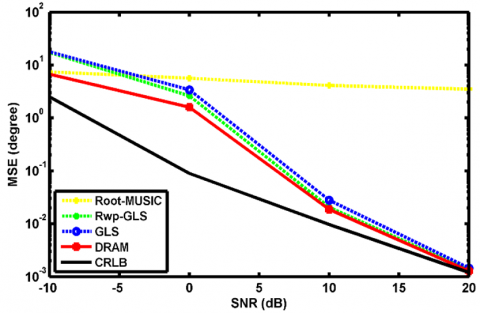
We first test the performance of DRAM versus SNR for $\sigma_{\Omega}=[1,4,7.3,10,8,3.5,6]$. Consider three uncorrelated sources imping on CPA from θ ̃=[0.1, 0.167,0.3] with SNR ranging from -10 dB to 20 dB. The results are shown in Figure 2. Note that the first two DoAs are separated by only $\Delta \tilde{\theta}=\frac{1}{N M}$. As it is shown, DRAM has the lowest MSE among all methods, which indicates its superiority in separating spatially adjacent signals under violated separation conditions and heteroscedastic noise cases.
Figure 2. MSEs of Root-MUSIC, Rwp-GLS, GLS, DRAM, and CRLB with respect to SNR
Figure 3. CPU times comparisons of Root-MUSIC, Rwp-GLS, GLS and DRAM with respect to SNR.
Figure 3 demonstrates the CPU times of the experiments related to Figure 2. DRAM is the most time-consuming due to the SVD decomposition in each iteration. This drawback is balanced by the estimation accuracy. Particularly, the computational complexity increases slightly till SNR=10 dB, because of the $\sigma_{\Omega}$ estimation, and when SNR>10 dB, DRAM converges more rapidly, leading to a decrease in the number of iterations and the time usage.
We then evaluate the MSE with respect to 15≤L≤50. The simulation is carried out assuming $\widetilde{\boldsymbol{\theta}}=$ [0.1, 0.167,0.3], SNR=10dB and $\sigma_{\Omega}=[8,9,2,5,7,4,10]$. The results are shown in Figure 4. It can be concluded that DRAM performs the best throughout the examined range, and that only a few snapshots are required to resolve the sources with $\Delta \tilde{\theta}=\frac{1}{N M}$ precision. While Root-MUSIC has the highest snapshot threshold.
Figure 4. MSEs of Root-MUSIC, Rwp-GLS, GLS, DRAM, and CRLB with respect to the number of snapshots
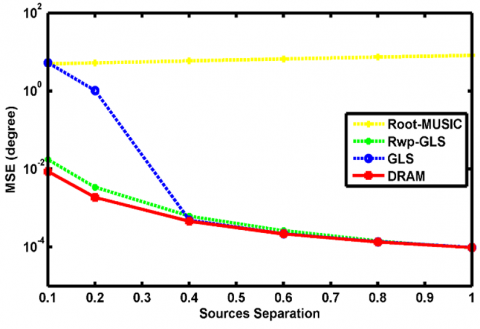
Figure 5. MSEs of Root-MUSIC, Rwp-GLS, GLS and DRAM with respect to the sources separations
To evaluate the performance of DRAM in terms of resolution, we test its ability in resolving closely spaced directions. Consider two signals impinge onto the CPA from $\widetilde{\boldsymbol{\theta}}=[0.1,0.1+\Delta \tilde{\theta}]$ with $\Delta \tilde{\theta} \in\left[\frac{0.1}{N M} \frac{1}{N M}\right]$, this corresponds to only 0.382° to 3.8° difference in angle. Our simulation results are presented in Figure 5 for SNR=10dB and $\sigma_{\Omega}=[8,9,2,5,7,4,10]$. The results indicate the superiority of DRAM over other methods in isolating spatially adjacent signals as close as $\frac{0.1}{N M}$ and thus exhibit super-resolution capability in DoA estimation.
In addition, to verify the robustness of the DRAM under heteroscedastic noise, the MSEs versus the WNPR are tested in Figure 6, in which WNPR ranges from 20 to 200, where SNR $\in${0, 10, 20} dB and $\widetilde{\boldsymbol{\theta}}=[0.1,0.3]$. It can be seen that for SNR=0 dB, the MSEs of both GLS and Rwp-GLS get larger than CRLB. In contrast to the MSEs of DRAM which coincides with CRLB for all values of SNR over the considered range of WNPR. This illustrates again the robustness of DRAM against the heteroscedastic noise.
Figure 6. MSEs of Rwp-GLS, GLS, DRAM and CRLB with respect to WNPR
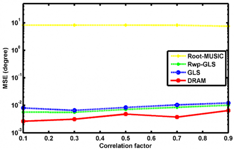
In the following, we provide an example to verify the ability of DRAM in resolving DoAs of correlated sources. Figure 7 shows the MSEs versus the correlation factor ρ, when SNR=10dB, $\sigma_{\Omega}=[8,9,2,5,7,4,10]$ and $\widetilde{\boldsymbol{\theta}}=$[0.1,0.167]. As shown, when the correlation factor increases DRAM shows immunity to the integrated correlations among sources and gains the best results.
Figure 7. MSEs of Root-MUSIC, Rwp-GLS, GLS and DRAM with respect to correlation factor
The problem of sparse gridless DoA estimation from compressive corrupted measurements was addressed in this paper. We present a hybrid optimization framework based on introducing CF criterion and nonconvex relaxation into the ANM approach. Then, an iterative reweighted minimization method is developed.
The effectiveness of the proposed method is verified through numerical simulations. The results have demonstrated the superiority of DRAM in isolating spatially adjacent signals as close as $\Delta \tilde{\theta}=\frac{0.1}{N M}$. As well, the results have shown that DRAM has the lowest snapshot threshold, and the best immunity against sources correlation and noise fluctuation among the compared methods. In the future, we may try more computationally efficient combining approach for noisy gridless DoA.
[1] Swindlehurst, A.L., Jeffs, B.D., Seco-Granados, G., Li, J. (2014). Academic Press Library in Signal Processing: Volume 3 - Array and Statistical Signal Processing. Academic Press Library in Signal Processing. https://doi.org/10.1016/c2013-0-00294-0
[2] Schmidt, R.O. (1981). A signal subspace approach to multiple emitter location and spectral estimation. PhD Thesis, Stanford University, California. Schmidt, R.
[3] Roy, R., Kailath, T. (2009). ESPRIT-Estimation of signal parameters via rotational invariance techniques. Adaptive Antennas for Wireless Communications, 37(7): 984-995. https://doi.org/10.1109/9780470544075.ch2
[4] Donoho, D.L. (2006). Compressed sensing. IEEE Transactions on Information Theory, 52(4): 1289-306. https://doi.org/10.1109/TIT.2006.871582
[5] Baraniuk, R.R.G. (2007). Compressive sensing. Signal Processing Magazine, 24(4). https://doi.org/10.1109/msp.2007.4286571
[6] Chae, D.H., Sadeghi, P., Kennedy, R.A. (2010). Effects of basis-mismatch in compressive sampling of continuous sinusoidal signals. Proceedings of the 2010 2nd International Conference on Future Computer and Communication, ICFCC 2010, pp. V2-739. https://doi.org/10.1109/icfcc.2010.5497605
[7] Chi, Y., Scharf, L.L., Pezeshki, A., Calderbank, A.R. (2011). Sensitivity to basis mismatch in compressed sensing. IEEE Transactions on Signal Processing, 59(5): 2182-2195. https://doi.org/10.1109/TSP.2011.2112650
[8] Li, Y., Chi, Y. (2016). Off-the-grid line spectrum denoising and estimation with multiple measurement vectors. IEEE Transactions on Signal Processing, https://doi.org/10.1109/TSP.2015.2496294
[9] Tan, Z., Nehorai, A. (2014). Sparse direction of arrival estimation using co-prime arrays with off-grid targets. IEEE Signal Processing Letters. https://doi.org/10.1109/LSP.2013.2289740
[10] Pal, P., Vaidyanathan, P.P. (2014). A grid-less approach to underdetermined direction of arrival estimation via low rank matrix denoising. IEEE Signal Processing Letters, 21(6): 737-741. https://doi.org/10.1109/LSP.2014.2314175
[11] Yang, Z., Xie, L. (2017). On gridless sparse methods for multi-snapshot direction of arrival estimation. Circuits, Systems, and Signal Processing, 36(8): 3370-3384. https://doi.org/10.1007/s00034-016-0462-9
[12] Chandrasekaran, V., Recht, B., Parrilo, P.A., Willsky, A.S. (2012). The convex geometry of linear inverse problems. Foundations of Computational Mathematics, 12(6): 805-849. https://doi.org/10.1007/s10208-012-9135-7
[13] Candès, E.J., Fernandez-Granda, C. (2014). Towards a mathematical theory of super-resolution. Communications on Pure and Applied Mathematics, 67(6): 906-956. https://doi.org/10.1002/cpa.21455
[14] Fernandez-Granda, C. (2015). Super-resolution of point sources via convex programming. 2015 IEEE 6th International Workshop on Computational Advances in Multi-Sensor Adaptive Processing, CAMSAP 2015, pp. 41-44. https://doi.org/10.1109/camsap.2015.7383731
[15] Tang, G., Bhaskar, B.N., Shah, P., Recht, B. (2013). Compressed sensing off the grid. IEEE Transactions on Information Theory, 59(11): 7465-7490. https://doi.org/10.1109/TIT.2013.2277451
[16] Candès, E.J., Fernandez-Granda, C. (2013). Super-Resolution from Noisy Data. Journal of Fourier Analysis and Applications. https://doi.org/10.1007/s00041-013-9292-3
[17] Bhaskar, B.N., Tang, G., Recht, B. (2013). Atomic norm denoising with applications to line spectral estimation. IEEE Transactions on Signal Processing, 61(23): 5987-5999. https://doi.org/10.1109/TSP.2013.2273443
[18] Yang, Z., Xie, L. (2016). Exact joint sparse frequency recovery via optimization methods. IEEE Transactions on Signal Processing, 64(19): 5145-5157. https://doi.org/10.1109/TSP.2016.2576422
[19] Tang, G., Bhaskar, B.N., Recht, B. (2015). Near minimax line spectral estimation. IEEE Transactions on Information Theory. https://doi.org/10.1109/TIT.2014.2368122
[20] Li, Q., Tang, G. (2020). Approximate support recovery of atomic line spectral estimation: A tale of resolution and precision. Applied and Computational Harmonic Analysis. https://doi.org/10.1016/j.acha.2018.09.005
[21] Yang, Z., Xie, L. (2015). On gridless sparse methods for line spectral estimation from complete and incomplete data. IEEE Transactions on Signal Processing, 63(12): 3139-3153. https://doi.org/10.1109/TSP.2015.2420541
[22] Wu, X., Zhu, W.P., Yan, J., (2017). A toeplitz covariance matrix reconstruction approach for direction-of-arrival estimation. IEEE Transactions on Vehicular Technology, pp. 8223-8237. https://doi.org/10.1109/tvt.2017.2695226
[23] Wu, X., Zhu, W.P., Yan, J. (2018). A high-resolution DOA estimation method with a family of nonconvex penalties. IEEE Transactions on Vehicular Technology, 67(6): 4925-4938. https://doi.org/10.1109/TVT.2018.2817638
[24] Yang, Z., Xie, L. (2016). Enhancing sparsity and resolution via reweighted atomic norm minimization. IEEE Transactions on Signal Processing, 64(4): 995-1006. https://doi.org/10.1109/TSP.2015.2493987
[25] Zien Alabideen, L., Al-Dakkak, O., Khorzom, K. (2019). Frequency recovery resolution enhancement using generalized reweighted nonconvex relaxation. U.P.B. Sci. Bull., Series C., 81(1): 81-98.
[26] Tan, W., Feng, X. (2019). Covariance matrix reconstruction for direction finding with nested arrays using iterative reweighted nuclear norm minimization. International Journal of Antennas and Propagation 2019. https://doi.org/10.1155/2019/7657898
[27] Lu, C., Tang, J., Yan, S., Lin, Z. (2014). Generalized nonconvex nonsmooth low-rank minimization. Proceedings of the IEEE Computer Society Conference on Computer Vision and Pattern Recognition, pp. 4130-4137. https://doi.org/10.1109/cvpr.2014.526
[28] Malek-Mohammadi, M., Babaie-Zadeh, M., Skoglund, M. (2015). Performance guarantees for Schatten-p quasi-norm minimization in recovery of low-rank matrices. Signal Processing, 114(C): 225-230. https://doi.org/10.1016/j.sigpro.2015.02.025
[29] Alabideen, L.Z., Al-Dakkak, O., Khorzom, K. (2020). Reweighted covariance fitting based on nonconvex schatten-p minimization for gridless direction of arrival estimation. Mathematical Problems in Engineering, 2020: 1–11. https://doi.org/10.1155/2020/3012952
[30] Zhou, C., Gu, Y., Zhang, Y.D., Shi, Z., Jin, T., Wu, X. (2017). Compressive sensing-based coprime array direction-of-arrival estimation. IET Communications, 11(11): 7465-7490. https://doi.org/10.1049/iet-com.2016.1048
[31] Tan, Z., Eldar, Y.C., Nehorai, A. (2014). Direction of arrival estimation using co-prime arrays: A super resolution viewpoint. IEEE Transactions on Signal Processing, 62(21): 5565-5576. https://doi.org/10.1109/TSP.2014.2354316
[32] Stoica, P., Babu, P., Li, J. (2011). New method of sparse parameter estimation in separable models and its use for spectral analysis of irregularly sampled data. IEEE Transactions on Signal Processing. https://doi.org/10.1109/TSP.2010.2086452
[33] Lin, B., Zhu, J. (2017). Sparse continuous-field and super-resolution method for direction-of-arrival estimation. Multidimensional Systems and Signal Processing. https://doi.org/10.1007/s11045-016-0451-y
[34] Blu, T., Dragotti, P.L., Vetterli, M., Marziliano, P., Coulot, L. (2008). Sparse sampling of signal innovations. IEEE Signal Processing Magazine. https://doi.org/10.1109/msp.2007.914998
[35] Barabell, A.J. (1983). Improving the resolution performance of eigenstructure-based direction-finding algorithms. ICASSP, IEEE International Conference on Acoustics, Speech and Signal Processing - Proceedings, pp. 336-339. https://doi.org/10.1109/icassp.1983.1172124
[36] Yang, Z., Li, J., Stoica, P., Xie, L. (2017). Sparse methods for direction-of-arrival estimation. Academic Press Library in Signal Processing, Volume 7: Array, Radar and Communications Engineering, pp. 509-581. https://doi.org/10.1016/b978-0-12-811887-0.00011-0
[37] Gu, S., Xie, Q., Meng, D., Zuo, W., Feng, X., Zhang, L. (2017). Weighted nuclear norm minimization and its applications to low level vision. International Journal of Computer Vision, 121(2): 183-208. https://doi.org/10.1007/s11263-016-0930-5
[38] Toh, K.C., Todd, M.J., Tütüncü, R.H. (1999). SDPT3 - a MATLAB software package for semidefinite programming, version 1.3. Optimization Methods and Software. https://doi.org/10.1080/10556789908805762
[39] Grant, M., Boyd, S. (2017). CVX: Matlab software for disciplined convex programming, ver 2.1. Available at Http://Cvxr.Com/Cvx/.
[40] Pesavento, M., Gershman, A.B. (2001). Maximum-likelihood direction-of-arrival estimation in the presence of unknown nonuniform noise. IEEE Transactions on Signal Processing, 49(7): 1310-1324. https://doi.org/10.1109/78.928686
[41] He, Z.Q., Shi, Z.P., Huang, L. (2014). Covariance sparsity-aware DOA estimation for nonuniform noise. Digital Signal Processing: A Review Journal, 28(1): 75-81. https://doi.org/10.1016/j.dsp.2014.02.013