Usha Mukkamala* | Srinivasa Rao Gunji
© 2020 IIETA. This article is published by IIETA and is licensed under the CC BY 4.0 license (http://creativecommons.org/licenses/by/4.0/).
OPEN ACCESS
Cutting force is an important measurement in machining to predict the life a tool and to estimate the power required. Standard mathematical models can be used to minimise the cutting forces (Fz). A comparative study is made in modelling the cutting force (Fz) through L18 and ANN models, while turning of AISI 1040 steel with tungsten carbide cutting insert. The input parameters that are considered are volume concentration, MQL flow rate, speed, feed and DOC The experiments were carried out using L18 Taguchi design process, and the analysis was made using SPSS to determine the model adequacy and also the influencing parameters effecting cutting force. Multi-Layer Perceptron (MLP) which is a class of feedforward artificial neural network was adopted to develop the mathematical prediction models. The predictive capabilities of L18 and ANN models were further compared in terms of their mean absolute percentage error. The results concluded that the ANN model is better in predicting the response with 3.78% mean absolute percentage error where as L18 model has an average percentage error of 7.58%. It was observed that the cutting force was reduced through ANN method by 7.814% when compared to L18 model. Both the models were used to further optimise the cutting force Fz through genetic algorithm. The results showed that the ANN model predicted optimal cutting force already, and the usage of genetic algorithm as a post processing step did not improve it any further.
MQL, nano cutting fluids, modelling, optimization, genetic algorithm, artificial neural networks
Various process parameters and machining performance (responses) are captured during machining process. In order to understand the relation and predict future responses, mathematical modelling is used. Mathematical models are usually developed based on experimental data using conventional methods like regression technique [1] used response surface methodology to predict the surface roughness in grinding operation and concluded that the model is adequate in estimating the response. Fratila and Caizar [2] in their paper stated that regression models are suitable for finding the relation between input variables and output responses. Lazir et al. [3] predicted the tool life in terms of both first order and second order models. Though both the models are valid in predicting the response, second order models have less average percentage error in prediction. Cakir et al. [4] in their paper developed linear model, second order model and exponential order model for surface roughness. The authors concluded that second order models are best in predicting the response with small errors compared to linear models. Linear regression models do not accurately reflect the non-linear relationship between the parameters and responses, leading to increased error in prediction. In these scenarios, non-conventional approaches like Artificial Neural Network (ANN) are also being used to predict responses where the conventional mathematical models are not effective in predicting the response accurately. ANN is a computer-based modelling technique based on statistical approach, and being increasingly used in many fields of engineering for modelling complex relationships between input parameters and output responses. Abbas et al. [5] developed a surface roughness model using ANN with a prediction accuracy of 1.35%. Ezugwu et al. [6] developed ANN model for various responses and build a relation between input parameters and responses. Zain et al. [7] developed regression and ANN model for predicting surface roughness and reduced the surface roughness by 1.57% and 1.05% respectively. Thus the authors concluded that regression model is better than ANN. Zerti et al. [8] developed 3 different models (L27, RSM and ANN) for surface roughness and showed that ANN models are better in prediction followed by RSM and Taguchi techniques. Abbas et al. [9] proposed a new optimisation method edge worth- pareto to optimise surface roughness while developing a model with ANN. Mukherjee and Ray [10] made a review on different mathematical models and suggested a systematic approach to optimise the process parameters in metal cutting operation.
Cutting fluids are an important part of machining process, where they reduce friction, improve the surface finish and prolong the tool-life [11]. However, the cutting fluids add to the cost, and are difficult to dispose due to environmental hazards and statutory regulation. For this reason, traditional wet lubrication is increasingly being replaced with minimum quantity lubrication (MQL). In MQL, a cutting fluid is converted to a fine mist using highly pressurized air. Various researchers conducted the study on MQL and concluded that MQL machining is the most efficient machining in reducing the cutting forces, surface roughness and to increase the tool life [12-17]. More recently, nano-particle based cutting fluids are gaining importance due to their superior properties over conventional fluids. Nano-fluids have been shown to improve surface finish, tool-life and thermal conductivity, while reducing cutting forces [18-22]. There are various parameters related to a nano-fluid that can be modelled and optimised for a specific machining operation. Some of the parameters are the size of the nano particles, type of nano particles and the volume concentration (%) of the nano-particles in a base fluid.
Though research is conducted using ANN technique less work is carried in comparison of regression and ANN techniques. The novelty of the work lies in application of genetic algorithm for regression and ANN models under nano MQL systems.
In this study, both regression technique and ANN technique were used to develop models for an experimental data set using nano-fluids in machining through minimum quantity lubrication (MQL). The predicted responses were optimised using genetic algorithm, and results from both techniques are compared.
2.1 Experimental prerequisites
Five parameters namely volume concentration (vol. conc), MQL flow rate, speed, feed and DOC (depth of cut) were considered for modelling and optimising the machining process while turning AISI 1040 steel with TNMG160408H tool insert under Minimum Quantity Lubrication (MQL) conditions using Al2O3 nano-cutting fluids. Al2O3 nano-particles of size 30nm were procured from Aarshadhaatu Green Nanotechnologies India Pvt Ltd. The nano-particles were mixed in base fluid of deionized water, and the resultant mixture was sonicated using ultrasound to generate a colloidal suspension of nano-fluid that was used for the machining operation using MQL. The mixture of nano-particles were varied in terms of volumetric concentration of 0.2%, 0.4% and 0.6% to generate 3 different types of nano-fluid. The experiments were planned to be conducted on a variable speed precision lathe machine with MQL set up as shown in Figure 1. The cutting forces in machining operation are very important to predict the life of cutting tool. The thermal analysis of the forces helps to estimate the power required. The main cutting forces (Fz) were measured using Kistler piezoelectric dynamometer. The various machining input parameters and their ranges are shown in the Table 1.
Table 1. Machining parameters and their levels
|
Factor symbol |
Factor |
Level 1 (-1) |
Level 2 (0) |
Level 3 (+1) |
|
A |
Volume Concentration (%) |
0.2 |
0.4 |
0.6 |
|
B |
MQL Flow rate(ml/min) |
3 |
4 |
5 |
|
C |
Cutting Speed Vc(m/min) |
80 |
100 |
120 |
|
D |
Feed Rate f (mm/rev) |
0.051 |
0.102 |
0.153 |
|
E |
DOC d (mm) |
0.25 |
0.5 |
0.75 |
Figure 1. Experimental set-up
2.2 Experiment design
In practice, the Design of experiment (DOE) method has been used quite successfully in several industrial applications as in optimising manufacturing processes. Optimising manufacturing process has been a key goal in several industrial applications, and design of experiments (DOE) method was used very successfully. Taguchi’s L18 orthogonal array was chosen for the current design as it requires less experimental trials. This is also quite efficient for handling more factors than traditional full factorial design. L18 experimental layout with response cutting force (Fz) are shown in Table 2.
Table 2. Experimental design with response cutting force (Fz)
|
S. No |
Vol. conc |
MQL flow rate |
Speed |
Feed |
DOC |
Cutting force Fz (N) |
|
1 |
-1 |
-1 |
-1 |
-1 |
-1 |
37.1 |
|
2 |
-1 |
0 |
0 |
0 |
0 |
279.523 |
|
3 |
-1 |
1 |
1 |
1 |
1 |
469.3 |
|
4 |
0 |
-1 |
-1 |
0 |
0 |
157.25 |
|
5 |
0 |
0 |
0 |
1 |
1 |
392.06 |
|
6 |
0 |
1 |
1 |
-1 |
-1 |
243.86 |
|
7 |
1 |
-1 |
0 |
-1 |
1 |
292.9 |
|
8 |
1 |
0 |
1 |
0 |
-1 |
232.098 |
|
9 |
1 |
1 |
-1 |
1 |
0 |
208.28 |
|
10 |
-1 |
-1 |
1 |
1 |
0 |
325.1 |
|
11 |
-1 |
0 |
-1 |
-1 |
1 |
197.36 |
|
12 |
-1 |
1 |
0 |
0 |
-1 |
155.37 |
|
13 |
0 |
-1 |
0 |
1 |
-1 |
179.627 |
|
14 |
0 |
0 |
1 |
-1 |
0 |
272.25 |
|
15 |
0 |
1 |
-1 |
0 |
1 |
312 |
|
16 |
1 |
-1 |
1 |
0 |
1 |
402.74 |
|
17 |
1 |
0 |
-1 |
1 |
-1 |
175.78 |
|
18 |
1 |
1 |
0 |
-1 |
0 |
230.31 |
3.1 Development of regression model
The model for cutting force was developed based on experimental data obtained from L18 design. The input parameters are provided in coded form and the analysis was carried out using SPSS statistical tool. R2 value of 0.958 shows that the input variables are able to predict the cutting force with 95.8% correlation [23]. ANOVA (Analysis of variance) is a statistical tool which is used to determine the model adequacy. ANOVA for cutting force and parameters effecting the cutting force are given in Tables 3 and 4, respectively.
Table 3. ANOVA for cutting force
|
Model |
Sum of squares |
Df |
Mean Square |
F |
Sig. |
|
Regression Residual Total |
175396.799 7615.380 183012.179 |
4 13 17 |
43849.200 585.798 |
74.584 |
0.000 |
Table 4. Coefficients of the parameters effecting cutting force
|
Model |
Unstandardized Coefficients |
Standardized Coefficients |
t |
Sig. |
|
|
B |
Std. Error |
Beta |
|||
|
(constant) MQLFlow rate Speed Feed DOC |
253.496 18.772 71.610 39.768 86.876 |
5.737 7.026 7.026 7.026 7.026 |
0.152 0.580 0.322 0.703 |
44.188 2.672 10.192 5.660 12.365 |
0.000 0.019 0.000 0.000 0.000 |
Table 5. Error percentage for predicted and experimental values
|
S. No |
Vol. conc |
MQL. flow rate |
Speed |
Feed |
DOC |
Predicted value |
Experimental values |
Error |
Error Percentage |
|
1 |
-1 |
-1 |
-1 |
-1 |
-1 |
36.47 |
37.1 |
0.63 |
1.698113 |
|
2 |
-1 |
0 |
0 |
0 |
0 |
253.496 |
279.523 |
26.027 |
9.311219 |
|
3 |
-1 |
1 |
1 |
1 |
1 |
470.522 |
469.3 |
1.222 |
0.260388 |
|
4 |
0 |
-1 |
-1 |
0 |
0 |
163.114 |
157.25 |
5.864 |
3.729094 |
|
5 |
0 |
0 |
0 |
1 |
1 |
380.14 |
392.06 |
11.92 |
3.040351 |
|
6 |
0 |
1 |
1 |
-1 |
-1 |
217.234 |
243.86 |
26.626 |
10.91856 |
|
7 |
1 |
-1 |
0 |
-1 |
1 |
281.832 |
292.9 |
11.068 |
3.778764 |
|
8 |
1 |
0 |
1 |
0 |
-1 |
238.23 |
232.098 |
6.132 |
2.641987 |
|
9 |
1 |
1 |
-1 |
1 |
0 |
240.426 |
208.28 |
32.146 |
15.43403 |
|
10 |
-1 |
-1 |
1 |
1 |
0 |
346.102 |
325.1 |
21.002 |
6.460166 |
|
11 |
-1 |
0 |
-1 |
-1 |
1 |
228.994 |
197.36 |
31.634 |
16.02858 |
|
12 |
-1 |
1 |
0 |
0 |
-1 |
185.392 |
155.37 |
30.022 |
19.32291 |
|
13 |
0 |
-1 |
0 |
1 |
-1 |
187.616 |
179.627 |
7.989 |
4.44755 |
|
14 |
0 |
0 |
1 |
-1 |
0 |
285.338 |
272.25 |
13.088 |
4.807346 |
|
15 |
0 |
1 |
-1 |
0 |
1 |
287.534 |
312 |
24.466 |
7.841667 |
|
16 |
1 |
-1 |
1 |
0 |
1 |
393.21 |
402.74 |
9.53 |
2.366291 |
|
17 |
1 |
0 |
-1 |
1 |
-1 |
134.778 |
175.78 |
41.002 |
23.32575 |
|
18 |
1 |
1 |
0 |
-1 |
0 |
232.5 |
230.31 |
2.19 |
0.950892 |
|
|
|
|
|
|
|
||||
|
|
|
|
|
|
|
Avg error |
7.575758 |
The regression equation for cutting force (N) is obtained from the coefficient values and is given in Eq. (1):
CF=253.496+18.772*Flowrate+71.610*Speed+39.768*feed+86.876*DOC (1)
Eq. (1) is used to predict the values of the cutting force (Fz). The percentage error is obtained between the experimental values and predicted values which are tabulated in Table 5.
Figure 2. Experiment vs Predicted values for cutting force
From Table 5 it is clear that the errors in predicting the cutting force are within the acceptable range. The same conclusion can be drawn from the line graph of experimental and predicted values of cutting force in Figure 2.
3.2 Computation of ANN model
Artificial neural networks (ANN) are computer models developed based on principles similar to how animal/human brains work. An ANN is modelled as a collection of artificial neurons (or) nodes, that are connected with other nodes with edges. Each node and edge have associated weights, which determine the output as a non-linear function of the inputs and weights. These weights are adjusted based on a training set of data (input and actual output). After the network is trained, the model can be used to predict the output for unknown inputs. There are multiple factors that are used / can be varied in development of ANN models for specific applications. Some of the most important factors are the network architecture or topology, activation functions used by the neurons, and the learning algorithm which is used to find the optimal values of weights. There are two types of network architecture, namely feedforward, and feedback neural networks. Feed forward neural networks are more popular. Signals travel only in one direction, i.e., from input to output. There are no cycles in the directed acyclic graphs [24]. Whereas, in the feedback network, the signals can also traverse from output to input, leading to cycles in the directed acyclic graphs [25].
The data should be normalized in order to get the best accurate network. Normalization of data was done using Eq. (2) [26]:
$X_{i}=\frac{\max y_{i}-y_{i}}{\max y_{i}-\min y_{i}}$ (2)
where, Xi is the normalised data for ith experiment. max(yi) and min(yi) are the maximum and minimum values of yipresent in the data set. The normalised values were calculated using Eq. (2) and used as target values while creating the network.
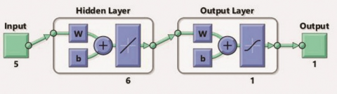
Initially several networks were build based on trial and error method for finding the best parameter settings to form a suitable network. The criteria for selecting the best network is to obtain the least Mean Square Error (MSE). The best network is obtained while using the Levenberg-Marquadt (LM) algorithm for training the network. The network was designed as a feed forward network with 6 neurons in the hidden layer for 5 input parameters and 1 output response. The network architecture is shown in Figure 3.
Figure 3. ANN with 6 neurons in hidden layer
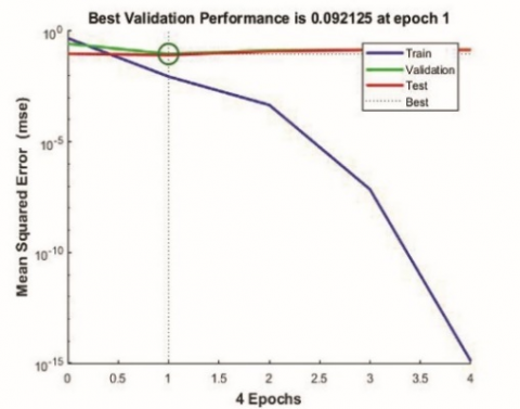
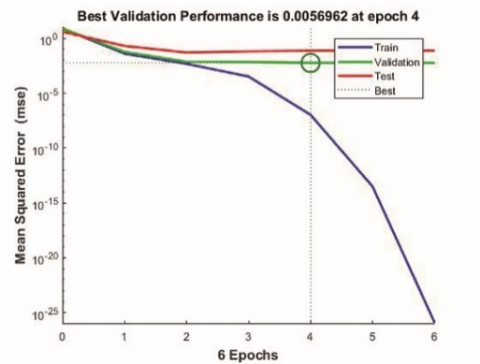
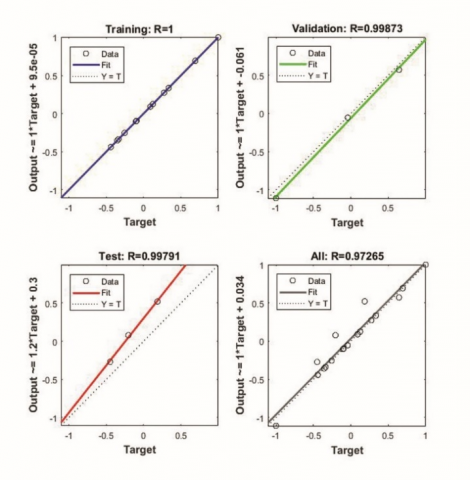
At first, the optimum number of neurons required was determined based on Mean Square Error (MSE). Options of 5, 6 and 7 neurons were tried and a size of 6 neurons was found to be optimal with low MSE. The overall R value which represents the correlation between training data and predicted values for network were 0.92427, 0.97265 and 0.89647 respectively for 5, 6 and 7 neurons. The performance graphs of the networks with 5,6 and 7 neurons indicating the MSE are shown in Figure 4.
From Figure 4 it is clear that network with 6 neurons in hidden layer has the least mean square error of 0.0056962 and hence are considered as the optimum number of neurons for constructing the network.
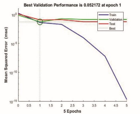
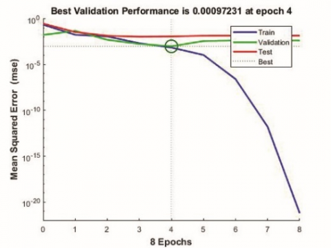
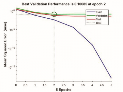
The input data from experiments can be divided into 3 different groups training, validation and testing. Training datasets are used for training the model. Validation datasets are used to measure network generalization and to halt training if the generalization stops improving. Testing datasets are used to check the predicted values and error in prediction based on actual data. These samples don’t have any effect on training. To check the efficiency of the network by improving the generalisation of network, 3 different percentages of validation data were considered as shown in Table 6. The mean square error and R values for 3 networks are shown in Figure 5 and Figure 6 respectively.
Table 6. Percentage of data used for training, validation and testing
|
Option |
Training data (%) |
Validation data (%) |
Testing data (%) |
|
1 |
80 |
10 |
10 |
|
2 |
70 |
15 |
15 |
|
3 |
60 |
20 |
20 |
(a) 5 neurons
(b) 6 neurons
(c) 7 neurons
Figure 4. Performance of ANN
(a) 10% validation data
(b) 15% validation data
(c) 20% validation data
Figure 5. Performance graphs
From Figure 5 it can be noticed that as the percentage of validation data increases the mean square error increases. The reason might be less data available for training. If validation and testing data are 20% each (total 8) then the no. of samples in training data will be only 10 (60%) which is very small. In this case least mean square value 0.000972 is obtained while validating and testing 10% data and training 80% data.
(a) 10% validation data
(b) 15% validation data
(c) 20% validation data
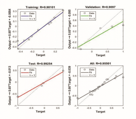
Figure 6. R values
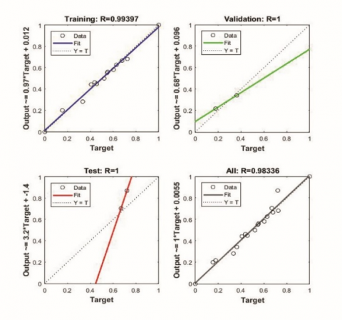
From Figure 6 it can be noticed that all the 3 networks have good R values for training, validation, testing and overall data. Highest overall R value (0.98336) which is close to 1 is obtained for the network with 10% validation and testing data and 80% training data.
Hence the network having 6 neurons in hidden layer and with 10% validation and testing data and 80% training data is considered as the optimum network. The predicted values from this network and the percentage error in predicting the values from the experimental values are presented in Table 7.
Table 7. Percentage error for Experimental Vs prediction through ANN
|
Predicted from ANN |
Experimental Values |
Error% |
|
36.16196 |
36.24 |
0.215329 |
|
269.3183 |
279.523 |
3.650759 |
|
470.6352 |
469.3 |
0.284514 |
|
151.2521 |
157.25 |
3.814261 |
|
375.559 |
392.06 |
4.208789 |
|
253.4652 |
243.86 |
3.93883 |
|
278.1725 |
292.9 |
5.028153 |
|
231.2845 |
232.098 |
0.35051 |
|
218.1477 |
208.28 |
4.737719 |
|
347.8663 |
325.1 |
7.002846 |
|
198.3892 |
197.36 |
0.521497 |
|
174.5593 |
155.37 |
12.35073 |
|
164.4595 |
179.627 |
8.443887 |
|
275.3883 |
272.25 |
1.152734 |
|
321.4408 |
312 |
3.025897 |
|
383.1957 |
402.74 |
4.852828 |
|
181.1767 |
175.78 |
3.070118 |
|
226.9261 |
230.31 |
1.469279 |
|
|
|
Average 3.784371 |
From Table 7 it is observed that the average error percentage in predicting the response from ANN is only 3.8%.
Genetic algorithm was used to optimise the response cutting force Fz. Genetic algorithm is one of the best optimisation tools to find the global optimum value. Genetic algorithms are developed from principles observed from nature, in particular, of natural genetics and natural selection. These algorithms try to map the desired optimal solution to the natural principle of the survival of the fittest. The set of possible solutions are modelled as an interbreeding population. An initial population is chosen and it is modelled over multiple generations, with genetic mutations and natural elimination, to finally converge on the optimal solution. Fitness function representing the relation between input variables and output response is chosen as part of a Genetic Algorithm. GA creates a set of initial population using the fitness function. The GA then iteratively creates new populations from the old by ranking the output responses and interbreeding the fittest to create new set of parameters that are expected to move closer to the optimum solution. In each generation, the GA creates a set of parameters, occasionally including new random data as mutations. Thus, the Genetic Algorithm can be used to model many different problems and obtain their optimal solutions [27].
A genetic algorithm starts with an initial population of random chromosomes or possible solutions. These solutions are evaluated with respect to their output, and are allowed to breed in such a way that those chromosomes which have better output are given more chances to reproduce. Occasionally some chromosomes are mutated similar to how mutations occur in nature. These are then filtered through principles of natural selection, so that the solutions with better characteristics continue to reproduce towards next generation, while chromosomes with poorer characteristics get eliminated via principles of natural selection. Thus, over many generations, the population gets better and better. When the population cannot get any better, the search is stopped and the current population is chosen as the optimal solution. Optimisation tool box from MATLAB was used to carry out the optimisation.
4.1 Optimisation using regression model
Eq. (1) which was obtained from regression of experimental data was used as a fitness function to formulate the problem in genetic algorithm. As there are five input parameters, five variables were considered with their ranges as lower and upper boundaries.
Problem definition:
Minimise
Fz=253.496+18.772*(x2)+71.610*(x3)
+39.768*(x4)+86.876*(x5)
where, x2, x3, x4 and x5 are MQL flow rate, speed, feed and DOC respectively.
Ranges of the parameters considered
-1 ≤ Volume concentration ≤ 1
-1 ≤ MQL flow rate ≤ 1
-1 ≤ Speed ≤ 1
-1 ≤ Feed rate ≤ 1
-1 ≤ DOC ≤ 1
The parameter settings for GA are given in Table 8.
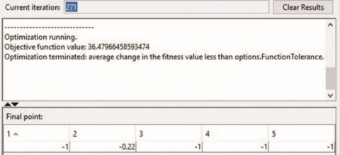
The results that were obtained after running the optimisation tool box is given in Figure 7. From Figure 7 it is found that optimum cutting force is 36.48N which is same as obtained from regression equation.
Table 8. Parameter settings in GA
|
Parameter |
Values |
|
Size of population |
100 |
|
Crossover rate |
0.7 |
|
Mutation rate |
0.1 |
|
No. of generations |
400 |
Figure 7. Optimum value for Cutting force through regression model
4.2 Optimisation using MLP model
The predicted values which are obtained from ANN were used to get the regression equation. The equation obtained for ANN predicted values is given below
CF=253.189+25.339*Flowrate+71.272*Speed+40.778*feed+82.19*DOC (3)
The Eq. (3) is considered as fitness function to optimise the response. and the results are displayed in Figure 8. From Figure 8 it is clear that the cutting force is optimised to 33.62kgf which is the least predicted value from ANN. After decoding, the optimum cutting force Fz is obtained at 0.57%, 3ml/min, 80m/min, 0.051mm/min and 0.25mm.
Figure 8. Optimum value for cutting force through ANN model
4.3 Comparison of regression and ANN models
The regression and ANN models were compared in terms of the optimised value obtained from GA. The results of comparison are shown in Table 9.
Table 9. Comparison of optimum values of regression and ANN models
|
Model |
Optimum value from GA |
Minimum value from model |
|
Regression |
36.47 |
36.47 |
|
ANN |
33.62 |
33.62 |
From Table 9 it is observed that cutting force cannot be further optimised through genetic algorithm for both ANN and L18 models.
(1) Equations are developed for cutting force for both L18 model and multi-layer perceptron model.
(2) Multi-layer perceptron model with 6 neurons in the hidden layer is considered as the best network.
(3) The percentage error in predicting the response for regression and MLP models are 7.58 and 3.78 respectively.
(4) Optimum cutting force obtained for regression and MLP models is 36.47N and 33.62N after application of GA.
(5) MLP model is better in predicting the response with less error and also to obtain the optimum cutting force compared to regression model.
(6) MLP model reduced the cutting force by 7.814% compared to L18 model.
|
F |
Cutting force, N |
|
V, x3 |
Speed, m/min |
|
F, x4 D, x5 |
Feed rate, mm/rev Depth of cut, mm |
|
R |
Dimensionless Regression |
|
Subscripts |
|
|
z |
Force acting along the z direction |
|
c |
Cutting speed |
[1] Kamely, M.A., Kamil, S.M., Chong, C.W., Grinding, A. (2011). Mathematical modeling of surface roughness in surface grinding operation. CiteSeerX.psu:10.1.1.294.1232
[2] Frǎţilǎ, D., Caizar, C. (2012). Investigation of the influence of process parameters and cooling method on the surface quality of AISI-1045 during turning. Materials and Manufacturing Processes, 27(10): 1123-1128. https://doi.org/10.1080/10426914.2012.677905
[3] Lajis, M.A., Karim, A.N.M., Amin, A.K.M.N., Hafiz, A.M.K., Turnad, L.G. (2008). Prediction of tool life in end milling of hardened steel AISI D2. European Journal of Scientific Research, 21(4): 592-602. http://irep.iium.edu.my/26853/
[4] Cakir, M.C., Ensarioglu, C., Demirayak, I. (2009). Mathematical modeling of surface roughness for evaluating the effects of cutting parameters and coating material. Journal of Materials Processing Technology, 209(1): 102-109. https://doi.org/10.1016/j.jmatprotec.2008.01.050
[5] Abbas, A.T., Pimenov, D.Y., Erdakov, I.N., Taha, M.A., Soliman, M.S., El Rayes, M.M. (2018). ANN surface roughness optimization of AZ61 magnesium alloy finish turning: Minimum machining times at prime machining costs. Materials, 11(5): 808. https://doi.org/10.3390/ma11050808
[6] Ezugwu, E.O., Fadare, D.A., Bonney, J., Da Silva, R.B., Sales, W.F. (2005). Modelling the correlation between cutting and process parameters in high-speed machining of Inconel 718 alloy using an artificial neural network. International Journal of Machine Tools and Manufacture, 45(12-13): 1375-1385. https://doi.org/10.1016/j.ijmachtools.2005.02.004
[7] Zain, A.M., Haron, H., Qasem, S.N., Sharif, S. (2012). Regression and ANN models for estimating minimum value of machining performance. Applied Mathematical Modelling, 36(4): 1477-1492. https://doi.org/10.1016/j.apm.2011.09.035
[8] Zerti, A., Yallese, M.A., Meddour, I., Belhadi, S., Haddad, A., Mabrouki, T. (2019). Modeling and multi-objective optimization for minimizing surface roughness, cutting force, and power, and maximizing productivity for tempered stainless steel AISI 420 in turning operations. International Journal of Advanced Manufacturing Technology, 102(1-4): 135-157. https://doi.org/10.1007/s00170-018-2984-8
[9] Abbas, A.T., Pimenov, D.Y., Erdakov, I.N., Mikolajczyk, T., El Danaf, E.A., Taha, M.A. (2017). Minimization of turning time for high-strength steel with a given surface roughness using the Edgeworth–Pareto optimization method. International Journal of Advanced Manufacturing Technology, 93(5-8): 2375-2392. https://doi.org/10.1007/s00170-017-0678-2
[10] Mukherjee, I., Ray, P.K. (2006). A review of optimization techniques in metal cutting processes. Computers and Industrial Engineering, 50(1-2): 15-34. https://doi.org/10.1016/j.cie.2005.10.001
[11] El Baradie, M.A. (1996). Cutting fluids: Part1. charecterisation. Journal of Materials Processing Technology, 56(1-4): 786-797. https://doi.org/10.1016/0924-0136(95)01892-1
[12] Masoudi, S., Vafadar, A., Hadad, M., Jafarian, F. (2018). Experimental investigation into the effects of nozzle position, workpiece hardness, and tool type in MQL turning of AISI 1045 steel. Materials and Manufacturing Processes, 33(9): 1011-1019. https://doi.org/10.1080/10426914.2017.1401716
[13] Liao, Y.S., Lin, H.M. (2007). Mechanism of minimum quantity lubrication in high-speed milling of hardened steel. International Journal of Machine Tools and Manufacture, 47(11): 1660-1666. https://doi.org/10.1016/j.ijmachtools.2007.01.007
[14] Dhar, N.R., Ahmed, M.T., Islam, S. (2007). An experimental investigation on effect of minimum quantity lubrication in machining AISI 1040 steel. International Journal of Machine Tools and Manufacture, 47(5): 748-753. https://doi.org/10.1016/j.ijmachtools.2006.09.017
[15] Tasdelen, B., Wikblom, T., Ekered, S. (2008). Studies on minimum quantity lubrication (MQL) and air cooling at drilling. Journal of Materials Processing Technology, 200(1-3): 339-346. https://doi.org/10.1016/j.jmatprotec.2007.09.064
[16] Hwang, Y.K., Lee, C.M. (2010). Surface roughness and cutting force prediction in MQL and wet turning process of AISI 1045 using design of experiments. Journal of Mechanical Science and Technology, 24(8): 1669-1677. https://doi.org/10.1007/s12206-010-0522-1
[17] Sharma, V.S., Singh, G., Sorby, K. (2015). A review on minimum quantity lubrication for machining processes. Materials and Manufacturing Processes, 30(8): 935-953. https://doi.org/10.1080/10426914.2014.994759
[18] Khandekar, S., Sankar, M.R., Agnihotri, V., Ramkumar, J. (2012). Nano-cutting fluid for enhancement of metal cutting performance. Materials and Manufacturing Processes, 27(9): 963-967. https://doi.org/10.1080/10426914.2011.610078
[19] Saravanakumar, N., Prabu, L., Karthik, M., Rajamanickam, A. (2014). Experimental analysis on cutting fluid dispersed with silver nano particles. Journal of Mechanical Science and Technology, 28(2): 645-651. https://doi.org/10.1007/s12206-013-1192-6
[20] Chan, C.Y., Lee, W.B., Wang, H. (2013). Enhancement of surface finish using water-miscible nano-cutting fluid in ultra-precision turning. International Journal of Machine Tools and Manufacture, 73: 62-70. https://doi.org/10.1016/j.ijmachtools.2013.06.006
[21] Vasu, V., Kumar, K.M. (2011). Analysis of Nanofluids as Cutting Fluid in Grinding EN-31 Steel. Nano-Micro Letters, 3(November): 209-214. https://doi.org/10.3786/nml.v3i4.p209-214
[22] Nam, J.S., Lee, P.H., Lee, S.W. (2011). Experimental characterization of micro-drilling process using nanofluid minimum quantity lubrication. International Journal of Machine Tools and Manufacture, 51(7-8): 649–652. https://doi.org/10.1016/j.ijmachtools.2011.04.005
[23] Pattanayak, B., Mohapatra, S.S., Das, H.C. (2019). Mathematical modelling for low temperature batch drying of paddy using fluidised bed technology. International Journal of Mathematical Modelling and Numerical Optimisation, 9(1): 89-103. https://doi.org/10.1504/IJMMNO.2019.096919
[24] Oplatková, Z.K., Hološka, J., Šenkeřík, R. (2013). Steganography content detection by means of feedforward neural network. International Journal of Mathematical Modelling and Numerical Optimisation, 5(3): 184-190. https://doi.org/10.1504/IJICA.2013.055932
[25] Jafarian, A., Nia, S.M. (2013). Feedback neural network method for solving linear Volterra integral equations of the second kind. International Journal of Mathematical Modelling and Numerical Optimisation, 4(3): 225-237. https://doi.org/10.1504/IJMMNO.2013.056531
[26] Rallabandi, S.R., Srinivasa Rao, G. (2019). Assessment of Tribological Performance of Al-Coconut Shell Ash Particulate—MMCs using Grey-Fuzzy Approach. Journal of The Institution of Engineers (India): Series C, 100(1): 13-22. https://doi.org/10.1007/s40032-017-0388-4
[27] Benabdouallah, M., El Yakoubi, O., Bojji, C. (2017). Genetic algorithm hybridised by a guided local search to solve the emergency coverage problem. International Journal of Mathematical Modelling and NumericalOptimisation, 8(1): 23-41. https://doi.org/10.1504/IJMMNO.2017.083657