Sreerag Choorikkat* | Rajyalakshmi Gajjele | Mellacheruvu Naga Srinivas | Akella Venkata Suryanarayana Murty
© 2020 IIETA. This article is published by IIETA and is licensed under the CC BY 4.0 license (http://creativecommons.org/licenses/by/4.0/).
OPEN ACCESS
The world of competition is not always deterministic. Probabilistic approach is more relevant and practical in any competitive environments. The effect of random failure gate which usually comes in the way of anything that promotes the low quality and at the same time denies high quality to come up in a competition and having a probability distribution for an instant of time is discussed in the present article. For this purpose the article introduces a novel methodology using the outcome probability of each rank along with the newly added concept of position ratios with a view to study the possibility of making proper predictions in the competitive environment discussed. The study also extends to infinite rank model cases as well. Moreover, a case study has been conducted to predict the risk of appropriate forecasting of different quality level using the model developed. The article emphasized the impact of number of failure gate and their respective influence in the area of ascertaining production quality making use of the concept of position ratio along with the outcome probabilities, which in turn improves the decision making to foresee the possible product quality variations in any manufacturing system, after a specific tenure of production. The methodology developed here will definitely find its application in the area of designing some powerful Decision Support Systems (DSS), where competition is fundamentally concerned with.
competition, random failure gates, position ratios, forecasting, Decision Support Systems (DSS)
Competitions are possible through different modes of execution, it is not necessary that all the competitors compete in the same instant of time. If the competition carried out through different set of converging pools which results in an ultimate winner in the end, such competitions can be generally represented as step-wise competition. If there is only a pair of competitors in a pool such competitions are single step competitions. Compound step competitions are those which favour the all competitors compete at the same time. Compound steps are capable to produce an ultimate winner and also the absolute rank list. The step-wise competitions always come under the probabilistic region because of its uncertainty in intermediate positions.
The outcome probabilistic model for discrete finite rank may be can explained using the following equations,
$P_{d}(n)=\frac{\lambda \sum_{i=1}^{n-1} S\left(n_{i}\right)+\left(\frac{S}{2}-\lambda\right)_{i=n+1}^{M} S\left(n_{i}\right)}{S_{C_{2}}}$ (1)
$P_{C}(n)=\frac{\frac{\lambda}{f(n)} R_{M-2} f(n) \omega_{1}+\frac{\left(\frac{A}{2}-\lambda\right)}{f(n)} R_{M-2} f(n) \omega_{2}}{\frac{1}{2} R_{M-2} \int_{a a}^{b b} \int f(z) \cdot\left(f(x)-\left(\frac{1}{b-a}\right)\right) d z \cdot d x}$ (2)
where,
$\begin{array}{l}
\omega_{1}=\int_{a}^{n} f(x) d x-\left(\lim _{\Delta x \rightarrow 0} f(n) \cdot \Delta x\right) \\
\omega_{2}=\int_{n}^{b} f(x) d x-\left(\lim _{\Delta x \rightarrow 0} f(n) \cdot \Delta x\right)
\end{array}$
The Eqns. (1) and (2) represent the outcome probability of discrete frequency model $P_{d}(n)$ and continues frequency model $P_{c}(n)$ respectively.
$f(x) \text { and } f(z)$ represent frequency distributions corresponding to $x^{t h} \text { and } z^{t h}$ rank respectively.
$f(n)$ represents the frequency distribution of $n^{t h}$ rank.
$f(n) \cdot \Delta x$ represents the number of competitors having $n^{t h}$ rank ( $\Delta x$ being strip width).
$\lim _{\Delta x \rightarrow 0} f(n) \cdot \Delta x$ represents the area of the elementary strip which represents number of competitors in the elementary strip.
$A$ and $S$ represents total number of competitors in continuous frequency model and discrete model respecticely.
Where, $A=\int_{a}^{b} f(x) d x \text { and } S=\sum_{i=1}^{M} S\left(n_{i}\right)$
M represents total number of competitors.
$\lambda$ represents number of failure gates.
$R_{M}$ represents the number of possible competition arrangements for M competitors.
$R_{M-2}$ represents the number of possible competition arrangement for M competitors by keeping one competitor fixed in apposition.
$n_{1} \text { and } n_{2}$ represents number of competitors in front of $n^{t h}$ position and behind $n^{t h}$ position respectively.
Where, $M=n_{1}+n_{2}+1 \text { and } R_{M}=M_{C_{2}} \cdot R_{M-2}$ .
$P(n)$ represents the pass through probability of $n^{t h}$ rank.
$a$ and $b$ are lower and upper limits of rank.
The model used these equations to study the effect of dummy competitors, random failure gate model and the possibility of applying position ratio in futuristic forecasting of winner in a competition.
Gilboa’s et al. [1] Probability and Uncertainty in Economic Modelling, noticed some limitations of the Bayesian approach and also identified some other models which can be implemented as a better economic model. Scala’s [2] also noticed different terminologies in probabilistic economics as well as the basic probabilistic ideas in the economic studies using probability theory. Menzel [3], Hickman [4], and Floyd [5] explained application of advanced probabilistic ideas in the economical oriented topics such as random variable transformations, probabilistic distributions. Xia et al. [6] pointed out a new methodology for reliability measurement of a running manufacturing system which may or may not have sample size along with probability distribution. Senol [7] introduced the Poisson process approach to identify the degree for failure mode and effect in reliability analysis. Also a process reliability assessment with a Bayesian approach which can predict whether the process holds the quality reliability requirements was introduced by Lin [8]. Reliability Modelling and Optimization Strategy for Manufacturing System Based on RQR Chain done by He [9]. Bhamare et al. [10] pointed out the evolution of reliability engineering in the last six decades and the various statistical and mathematical models developed during this tenure.
Samuelson’s [11] Evolution and Game Theory is found to be one of the basic research articles for the application of evolutionary game theory in economic science. An asymmetric competition game model in E-Marketplace introduced by Zheng et al. [12] studies the competition between sellers and buyers together. Friedman’s [13] study is a fundamental intro-literature for the implementation of evolution game theory in modern economics. Ozkan-Canbolat et al. [14] concentrates on the circumstances in which the bandwagon diffusion of an innovation happens in a jointly even though, on an average, organizations in which jointly assess negative outcomes through adapting a particular innovation. Also a medical application of game theory was introduced by Bellomo and Delitala [15]. The analysis includes mathematical kinetic theory of active particles applied to the modelling of the very early stage of cancer phenomena. Wooldridge [16], Jormakka and Mölsä [17] studied the application of game theory in warfare. Jorswieck [18] mentioned another application of game theory in the field of signal processing and communication engineering. Noguchi et al. [19] obtained rational solution through game theory for a multi-objective electromagnetic apparatus. Anastasopoulos et al. [20] created a model which can be used as a feedback suppression system on a multicast-satellite. The impact of inactive dummy competitors and also the possibility of using identical probability theory is well explained in recent studies [21, 22]. Sreerag et al. [23], studied the concepts of infinite and discrete rank models in detail and provided the mathematical proof behind this novel mathematical philosophy introduced.
The limitation of using conventional game theory to handle more number of competitors at the same time and also the ignoring of the underlining competition behaviour in between the competitors, the inability of Bayesian approach to potentially find its role when multiple competitors are included in competition are some of the vast literature gapes existing. The model developed here resolves the DSS dilemma involved in two different spheres, one through the idea of number of failure gates impacting on the system and likewise, analysing the associated instantaneous position ratios of the competitors according to their positions.
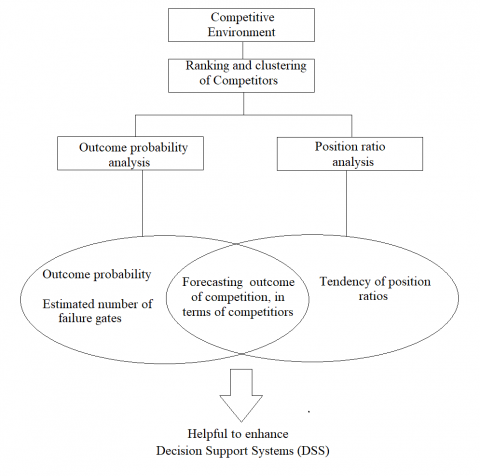
The flow chart representation of the methodology developed, and how it ultimately helps in the enhancement of Decision support system s (DSS) is provided in Figure 1.
Figure 1. Flow chart for the methodology of the study
Though the outcome probabilities along with the number of failure gate considered here gives the probability of ascertaining of a specific standard or quality, this may not itself explain the question of when it happens. However, by incorporating the concept of position ratios, the patterns of instantaneous position ratios, throughout the process period, help us to identify the possible convergence of our predictions more precisely. Earlier this has not been done so far. Hence it is imperative and really vital to consider the trends of position ratios as well, for better and accurate decision making.
The failure gate may not be deterministic for an instant of time. However, we can attach probabilistic distributions like normal, Poisson etc. to describe the possible pattern of failure gates. Figure 2 generally represents the expected probability distributions in such cases.
Figure 2. Possible probability distribution
Outcome probability of $n^{t h}$ rank in $\lambda$ failure gates $P(n / \lambda)$ which can be obtained from the Eq. (1). $P(n)$ is the probability of getting $n^{t h}$ position without the effect of failure gates, $P(\lambda)$ is the probability of happening a fixed number of failure gates which can be calculated from the probability distribution. $P(\lambda / n)$ is the probability of happening a fixed number of failure gates for $n^{t h}$ rank which is nothing but the effect-cause analysis of random failure gate distribution. On applying bayesian approach
$P(\lambda / n) \cdot P(n)=P(n / \lambda) \cdot P(\lambda)$ (3)
Let
$\begin{aligned}
&0 \leq P(\lambda / n) \leq(1 / \gamma) \text { where, } \gamma \geq 1\\
&0 \leq \frac{P(n / \lambda) \cdot P(\lambda)}{P(n)} \leq(1 / \gamma)\\
&0 \leq P(\lambda) \leq \frac{P(n)}{\gamma P(n / \lambda)}\\
&0 \leq P(\lambda) \leq(\eta / \gamma) \text { where, } \frac{P(n)}{P(n / \lambda)}=\eta
\end{aligned}$
where, $\eta$ is the ratio between outcome probability of $n^{t h}$ position without effect of failure gate, to the outcome probability of $n^{t h}$ position with failure gate.
If the probability of failure gates ranges from 0 to 1 then we come across the following situations.
Case (i): (when $\eta<1$ )
If the Outcome probability of $n^{t h}$ rank in $\lambda$ failure gates $P(n / \lambda)$ is greater than the probability of getting P(n / \lambda) position without the effect of failure gates $P(n)$ then
$P(\lambda / n)$ ranges from 0 to $1,0 \leq P(\lambda / n) \leq 1$ (4)
Case (ii): (when $\eta>1$ )
If the Outcome probability of $n^{t h}$ rank in $\lambda$ failure gates $P(n / \lambda)$ is smaller than the probability of getting $n^{t h}$ position without the effect of failure gates $P(n) \text { then } P(\lambda / n)$ ranges from 0 to $(1 / \eta)$ ,
$0 \leq P(\lambda / n) \leq(1 / \eta)$ (5)
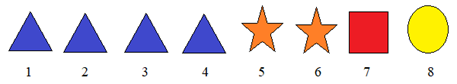
The system predictability is based on how the individual positions in a system helps in the whole prediction of the system. In this section, we are considering an example where system consists of 8 individual pictures distributed for various frequencies by their shapes (Figure 3). However, their position numbers fixed but all the members can be seated in any order and the observer is aware of these facts.
Figure 3. System with 8 individuals with various shape and colours with different numbers
If we know who is in the 1st, 2nd or 3rd or combined positions, then still there is an uncertainty to predict the whole system. The identification of 4th, 5th or 6th or combined positions may help you to the exact prediction of the system as a whole. The remaining two positions are the absolute predictable positions. This classification is as follows in the Table 1 given below.
Table 1. Different prediction status for different visible number of position
|
Position |
Status |
|
1st |
Unpredictable |
|
2nd |
Unpredictable |
|
3rd |
Unpredictable |
|
4th |
Predictable or Unpredictable |
|
5th |
Predictable or Unpredictable |
|
6th |
Predictable or Unpredictable |
|
7th |
Predictable |
|
8th |
Predictable |
The number of predictable or unpredictable position $N_{P / N}(t)$ can be computed as follows.
$N_{p / N}(t)=N_{L}(t)-1$ (6)
Now, the number of unpredictable positions $N_{L}(t)$ is computed by using the mathematical relationwhere, $N_{U P}(t)$ represents number assigned for the largest individual competitor.
$N_{U P}(t)=h(t)-\left(N_{L}(t)+1\right)$ (7)
where, $h(t)4 is the total number of competitors.
In the case of purely predictable, the number of predictable positions will be 2 for systems having more number of competitors.
The position ratio is the ratio between $N_{P / N}(t) \text { and } N_{L P}(t)$ which can be used as an indication of the predictability of the system for time t .
$\text { Therefore, Position ratio }=\frac{N_{P / N}(t)}{N_{U P}(t)}$ (8)
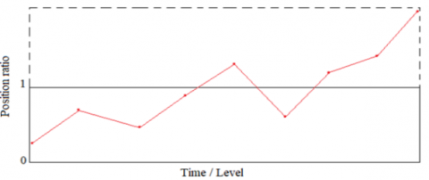
By comparing the position ratios with the instantaneous probabilities of different positions, one can estimate the tendency of the system as well as the futuristic forecasting of the winner, before the completion of the competition. The position ratio may tend to infinity in the case of elimination competition. i. e., finally only one competitor exists in the competition and all others disappear. The following Figure 4 is the expectation curve for position ratio for different time ‘t ’. The position ratio can be started from any value but converges to infinity for a single winner competition.
Figure 4. The expectation curve based on position ratio and time
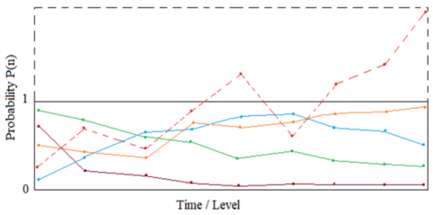
Figure 5. The outcome probability distributions for different competitors at different times (in non-elimination)
Figure 6. The outcome probability distributions for different competitors at different times (in elimination)
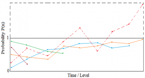
In the case non elimination competition, all the competitors have some valid outcome probabilities when the competition finished. The graphical representation of non-elimination competition with position ratio is shown in Figure 5.
In the case of elimination, the competitors get eliminated in each time period or level and only a single or few competitor reach the final position, refer Figure 6.
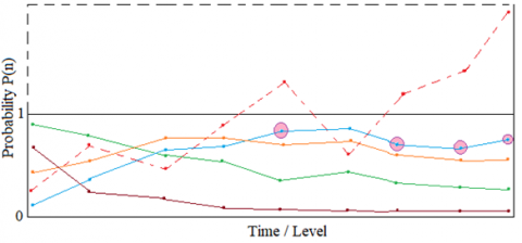
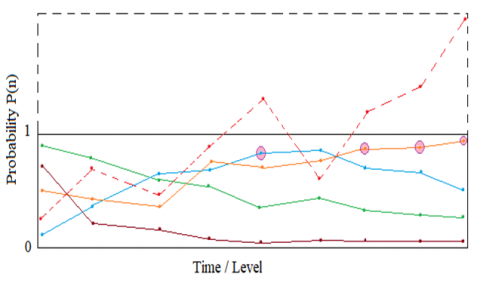
Now, we discuss about the convergence of a competitor to become winner. The study focused on high and low convergence of prediction probabilities in a competition. In the earlier discussion, it is mentioned that, initially the position ratios can assume any values. We can provide certain range for position ratios and hence higher and lower position ratios can be distinguished. Usually we can treat the range as 1, big value for high position ratio gives more accurate prediction but after certain limit this may reduce the possibility of predicting the winner. If the value of position ratio is high and a particular competitor showing high outcome probability throughout the time period, then such a competition can be classified under high convergence of prediction probability. However, if there is no such particular competitor have high outcome probability in the same time period then such a competition can be classified under low convergence of prediction probability. Usually we can treat this range as 1, big value for high position ratio gives more accurate prediction but after certain limit this may diminish the possibility of prediction. This analysis is also discussed graphically as shown in Figures 7-8.
Figure 7. High convergence of prediction probability in a competition
From Figure 7, it is clear that whenever position ratio is more than the range (=1), then outcome probability of blue coloured competitor found to be in the peak. Hence, we can conclude that competition have high convergence of prediction probability.
Figure 8. Low convergence of prediction probability in a competition
From Figure 8, it is clear that whenever position ratio is more than the range (=1), then outcome probability of blue and red coloured competitors found to be in the peak in different time periods. Hence it concluded that the competition has low convergence of prediction probability.
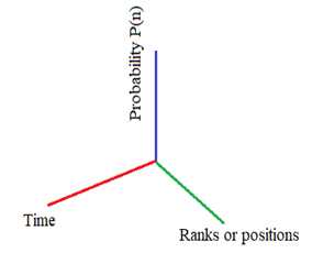
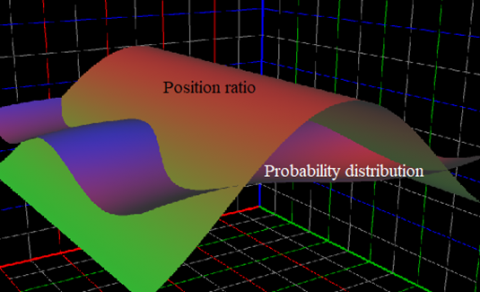
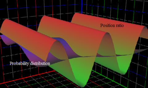
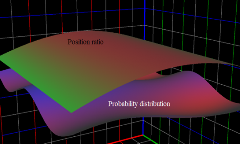
Similarly the same analysis can be implemented on infinite positions (ranks) with frequency distribution along with position ratio. The following figures representing the probability surface using 3D plotter software, with coordinates shown in Figure 9.
Figure 9. 3D coordinates for the current study
Figure 10. 3D view of probability distribution with fewer intersections
Figure 11. 3D view of probability distribution with more intersections
Figure 12. 3-dimensional view of probability distribution with no intersections
From Figure 10, it is clear that only few ranks having probability come under the higher range of position ratio. From Figure 11, more ranks having probability come under the higher range of position ratio. From Figure 12, none of the ranks having probability come under the higher range of position ratio.
The case study conducted below refers the application of this mathematical model in the quality control environment. The study makes use of the concept of six-sigma and developed the competition model in order to analyse the process in control or not and also consider and classify the region beyond six-sigma in terms of different number of failure gates. The study also extends for interpolating the number of failure gates in a specific time and also identifying the possibility of forecasting ensured process control in the long tenure using the cause- effect analysis discussed.
A clutch plate manufacturer has a variety of six quality standards with reference to the diameter tolerance of the clutch plates producing. The objective of the firm is to produce a 50cm diameter clutch plates. The table shown below (Table 2) represents these different standards based on their tolerance.
Table 2. Details regarding clutch plate
|
Diameter of the Clutch plate (cm) |
Range of tolerance (+ cm) |
Standard/ level/ rank |
|
50 |
0.1 - 0.2 |
1 |
|
50 |
0.2 – 0.3 |
2 |
|
50 |
0.3 – 0.4 |
3 |
|
50 |
0.4 – 0.5 |
4 |
|
50 |
0.5 – 0.6 |
5 |
|
50 |
0.6 – 0.7 |
6 |
The company is producing a total number of 1500 clutch plates per day. A sample of the products produced is inspected for the last 6 months. The sample’s frequency-rank distribution before inspection is shown below (Figure 13) for the first day of manufacturing with a sample size of 12 plates.
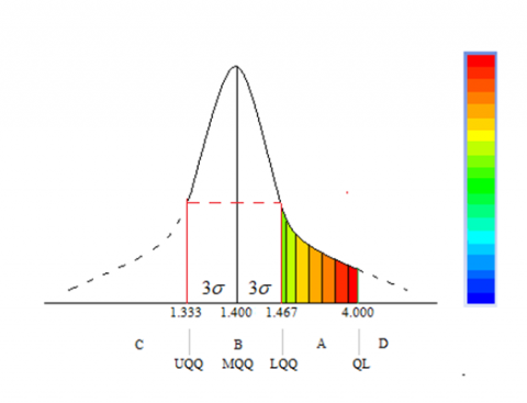
In this bar chart 2.33 is found to be best half quality of the manufacturing. let this value be called as the upper half quality (UHQ) and the best quarter quality is at 1.33, denoted as upper quarter quality (UQQ). The deviation from this UQQ will result in unreliable inspections. QL represents the least possible quality inspection where failure gates are in its maximum.
Figure 13. Inspection result for first day of manufacturing
For all values of number of failure gates there will be a fixed rank having a fixed probability in a constant rank-frequency distribution. If the outcome probability (from Eq. 1) of this particular position is almost near to 0.5 then consider this point as mean half quality (MHQ) (Figure 14). The half of this MHQ will give the mean quarter quality (MQQ).
Since for two different number of failure gates $\lambda_{i} \text { and } \lambda_{k}$ , the $n^{t h}$ portion where the better and worse halves get separated, while on substitution $\lambda_{i} \text { and } \lambda_{k}$ in Eq. (1), we get,
$\sum_{i=1}^{n-1} A\left(n_{i}\right)=\sum_{i=n+1}^{M} A\left(n_{i}\right)$ (9)
The $n_{i}$ in Eq. (9) represents the mean of the total clustered ranks and classifies the best half members and worst half members from the totality. Let us refer this as the mean half quality (MHQ).
Since the model developed is fundamentally built on competitions where the participating members having 50-50 chances of outcome realisation, hence, the maximum probability corresponding to MHQ is itself here resisted to 0.5. However, the rank corresponding to the MHQ can be anywhere physically.
Hence, this intersection of MHQ is mathematically possible and realistic as well.
Figure 14. Rank- probability distribution for different number of failure gates
Figure 15. Normally distributed quarter quality (QQ)
The quarter quality QQ is assumed to be normally distributed with the mean of MQQ and standard deviation $\sigma$ (Figure 15). On implementing 6 $\sigma$ , assuming the difference between MQQ and UQQ is 3 $\sigma$ . So, the difference between UQQ and LQQ is 6 $\sigma$ (named as zero failure gate region), where LQQ is the least quarter quality. The region between LQQ and QL is named as non-zero failure gate region.
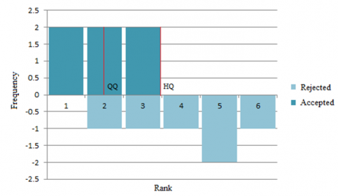
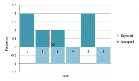
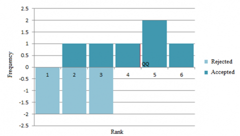
The Figures 16, 17, 18 shown below represent the outcome from inspectional unit after two, four, and six months respectively. HQ represents half quality and QQ represents quarter quality.
Figure 16. Inspection result on month 2
Figure 17. Inspection result on month 4
Figure 18. Inspection result on month 6
Since the total possible values of $\lambda$ ranges from 0 to 6 ie., $0 \leq \lambda \leq 6$ .
Thus, number of failure gates ( $\lambda$ ) can be expressed using the equation
$\lambda=\frac{M \cdot(Q Q-L Q Q)}{2 \cdot(Q L-L Q Q)}$ (10)
For this particular case study, we have,
$\begin{array}{c}
(Q L-L Q Q)=(4-1.467)=2.533 \\
\mathrm{N}=M=12 \text { (Sample size) }
\end{array}$
Therefore Eq. (1) becomes,
$\lambda=\frac{(Q Q-L Q Q)}{0.422167}$ (11)
The contribution to the number of failure gates in second, fourth and sixth month in the inspection unit in the expected situations (mentioned as remarks) is tabulated below (Table 3). The graph will help to forecast the possible number of failure gates for an instant of time. The model is the least economical way of conducting inspection with minimum number of inspectional trials.
Table 3. Impact of different number of failure gate in the system
|
Month |
Quarter quality (QQ) |
Number of failure gates (λ) |
Remarks |
|
Second |
1.5 |
0.0782 |
The production quality is excellent in nature. |
|
Fourth |
2 |
1.2625 |
Even though there is some reduction in the production quality, still the processes have a good performance. |
|
Sixth |
4 |
5.9999 |
Poor condition of production quality, almost all poor standards are producing in the production cycle. Red alert condition. |
5.1 Convergence of prediction probability in quality rankings
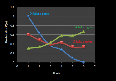
The prediction possibility of convergence can be analysed through the above mentioned procedure discussed earlier in section 4. The method makes use of the concept of position ratio (refer section 3 and 4). The value for the position $N(L) \quad, \quad N(P / N) \quad, \quad N(U P)$ and position ratio corresponding to different month is shown in Table 4.
Table 4. Position ratio obtained for different months
|
Month |
1st |
2nd |
3rd |
4th |
5th |
6th |
Total |
N(L)* |
N(P/N) |
N(UP) |
Position ratio |
|
1 |
2* |
2* |
2* |
0 |
0 |
0 |
6 |
2 |
1 |
3 |
0.333 |
|
2 |
2* |
1 |
1 |
0 |
2* |
0 |
6 |
2 |
1 |
3 |
0.333 |
|
3 |
0 |
1 |
1 |
1 |
2* |
1 |
6 |
2 |
1 |
3 |
0.333 |
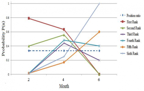
Figure 19. Outcome probability with position ratio for the 3 months
The outcome probability of each rank for the three different months is plotted in the Figure 19. From the Table 2 the value of position ratio 0.33 which is less than 1 indicate the high risk in forecasting a winner quality. Position ratio should be more than 1 to make a comfortable prediction. This highlights the complexity in forecasting the winner in advance.
It is clear from the Figure 19 that none of the ranks have proper leading edge throughout months. This represents the unstable outcome probability distribution of each rank. On account of the poor position ratio this unstable outcome probability distribution will result in a low convergence of prediction probability in the competition.
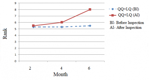
Figure 20. Rank-month plot for before and after inspection
The process control can be analysed through rank- month plot for the sum of QQ and QL before and after inspection in different months. The process is said to be in control if the deviation from the before and after (QQ + QL) is within $6 \sigma$ limit (Based on the design requirement). The rank- month plot is shown in the Figure 20.
Lower the value in QQ+QL (AI) on comparing to the QQ+QL (BI) is actually a good sign of quality production which indirectly represents very less poor quality in your production. However, higher the value in QQ+QL (AI) on comparing to the QQ+QL (BI) is the representation of poor quality production. Equal QQ+QL (AI), QQ+QL (BI) means the production is perfectly under control.
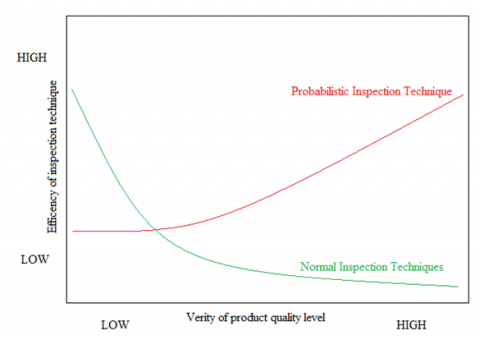
5.2 Comparison with normal quality control technique-Probabilistic inspection technique
The quality control technique introduced in this article is very relevant in the manufacturing scenario with high responsiveness. The high responsive inspection system considers wide range of quality levels based on normal techniques not incorporated with any methods to deal with wide variety of quality levels. Despite few limitations especially in the less or no verity quality level cases, the present model seems effective in the more general realm, where more verity of quality levels are considered. The Figure 21 compares the efficiency characteristics of probabilistic and normal inspection techniques. Probabilistic inspection model is relevant in cost effective inspection because it takes very less inspection trials compared to normal inspection techniques.
Figure 21. Comparison between normal and probabilistic inspection techniques
The effect of random failure gate in a competition having a probability distribution for an instant of time and the effect-cause probabilities are discussed. The method of comparing position ratios and outcome probability of each rank in order to predict or study the possibility of prediction is analysed and the effect of marginal value (range) of position ratio in the accuracy of prediction is discussed. The infinite rank model is also discussed in terms of position ratio. The study of infinite rank model may be useful in the field of particle science to study the probability to see a particle in a specific region. The same study of system predictability will help us to analyses prediction possibility in any general competitions including industrial competitions where competitors compete for a common target. A case study has been conducted and concluded that the model is practically mature enough in the decision making process especially in describing the possibility of forecasting outcome quality during inspection and also comparison on the benefits and limitations of probabilistic inspection technique with normal inspection techniques is done. This model will certainly find its application in the field of quality and inspection engineering, economics, social sciences and a wide variety of other areas of interest as well. From the case study (section 5) conducted, the observations made are as follows,
The methodology developed here is equally applicable on other areas of research relating to the competitions involved in-between suppliers in a supply chain management and the DSS in the same supply chain and the associated trust issues.
|
A |
Non-zero failure gate region |
|||
|
B |
Zero failure gate region |
|||
|
C D |
Impossible best quality region Impossible poor quality region |
|||
|
N UHQ UQQ MHQ MQQ LQQ QL HQ |
Sample size Quarter quality Upper half quality Upper quarter quality Mean half quality Mean quarter quality Lower quarter quality Quarter quality Half quality |
|||
|
Greek symbols |
|
|||
|
$\sigma$ |
Standard deviation of QQ |
|||
|
$\lambda$ |
Number of failure gates |
|||
[1] Gilboa, I., Postlewaite, A.W., Schmeidler, D. (2008). Probability and uncertainty in economic modeling. Journal of Economic Perspectives, 22(3): 173-88. https://doi.org/10.1257/jep.22.3.173
[2] Scalas, E. (2008). Introduction to probability theory for economists. Universita del Piemonte Orientale (Amedeo Avogadro). http://www.phdeconomics.sssup.it/documents/probpisanew.pdf, accessed on Oct. 22, 2008.
[3] Menzel, K. (2008). Economics Introduction to Statistical Methods in Economics. https://ocw.mit.edu/courses/economics/14-30-introduction-to-statistical-method-in-economics-spring-2006/index.htm.
[4] Hickman, B. (2009). Introduction to Probability Theory for Graduate Economics: Solutions to Chapter 1 Exercises. http://home.uchicago.edu/~hickmanbr/uploads/PT_REVIEW_CH1.pdf, accessed on Nov. 20, 2009.
[5] Floyd, J.E. (2010). Statistics for Economists: A Beginning. Toronto: University of Toronto, 1-292.
[6] Xia, X.T., Zhu, W.H., Liu, B. (2016). Reliability evaluation for the running state of the manufacturing system based on poor information. Mathematical Problems in Engineering, 2016: Article ID 7627641. https://doi.org/10.1155/2016/7627641
[7] Şenol, Ş. (2007). Poisson process approach to determine the occurrence degree in failure mode and effect reliability analysis. Quality Management Journal, 14(2): 29-40. https://doi.org/10.1080/10686967.2007.11918024
[8] Lin, G.H. (2005). Process reliability assessment with a Bayesian approach. The International Journal of Advanced Manufacturing Technology, 25(3-4): 392-395. https://doi.org/10.1007/s00170-003-1807-7
[9] He, Y., He, Z., Wang, L., Gu, C. (2015). Reliability modeling and optimization strategy for manufacturing system based on RQR chain. Mathematical Problems in Engineering, 2015. https://doi.org/10.1155/2015/379098
[10] Bhamare, S.S., Yaday, O.P., Rathore, A. (2008). Evolution of reliability engineering discipline over the last six decades: A comprehensive review. Int J Reliab Saf, 1(4): 377-410. https://doi.org/10.1504/IJRS.2007.016256
[11] Samuelson, L. (2002). Evolution and game theory. Journal of Economic Perspectives, 16(2): 47-66. https://doi.org/10.1257/0895330027256
[12] Zheng, J.Y., Li, W.G., Li, D.L. (2015). A Game-theory based Model for Analyzing E-marketplace Competition. In Proceedings of the 17th International Conference on Enterprise Information Systems - Volume 2: ICEIS, Barcelona, Spain, pp. 650-657. https://doi.org/10.5220/0005467706500657
[13] Friedman, D. (1998). On economic applications of evolutionary game theory. Journal of Evolutionary Economics, 8(1): 15-43. https://doi.org/10.1007/s001910050054
[14] Ozkan-Canbolat, E., Beraha, A., Bas, A. (2016). Application of evolutionary game theory to strategic innovation. Procedia-Social and Behavioral Sciences, 235: 685-693. https://doi.org/10.1016/j.sbspro.2016.11.069
[15] Bellomo, N., Delitala, M. (2008). From the mathematical kinetic, and stochastic game theory to modelling mutations, onset, progression and immune competition of cancer cells. Physics of Life Reviews, 5(4): 183-206. https://doi.org/10.1016/j.plrev.2008.07.001
[16] Wooldridge, M. (2012). Does game theory work? IEEE Intelligent Systems, 27(6): 76-80. https://doi.org/10.1109/MIS.2012.108
[17] Jormakka, J., Mölsä, J.V.E. (2005). Modelling information warfare as a game. Journal of Information Warfare, 4(2): 12-25.
[18] Jorswieck, E.A., Larsson, E.G., Luise, M., Poor, H.V. (2009). Game theory in signal processing and communications [from the guest editors]. IEEE Signal Processing Magazine, 26(5): 17-132. https://doi.org/10.1109/MSP.2009.933610
[19] Noguchi, S., Miyamoto, T., Matsutomo, S. (2014). Meaning of the rational solution obtained by game theory in a multi-objective electromagnetic apparatus design problem. IEEE Transactions on Magnetics, 50(2): 649-652. https://doi.org/10.1109/TMAG.2013.2281848
[20] Anastasopoulos, M.P., Taleb, T., Cottis, P.G., Obaidat, M.S. (2012). Feedback suppression in multicast satellite networks using game theory. IEEE Systems Journal, 6(4): 657-666. https://doi.org/10.1109/JSYST.2012.2192755
[21] Srinivas, M.N., Sreerag, C., Murty, A.V.S.N. (2019). Impact of dummy variables in a probabilistic competitive environment. SN Applied Sciences, 1(9): 1115. https://doi.org/10.1007/s42452-019-1121-0
[22] Sreerag, C., Srinivas, M.N., Murty, A.V.S.N. (2020). Modelling and outcome analysis of a competitive environment–A probabilistic approach (in press). Journal of King Saud University-Engineering Sciences. https://doi.org/10.1016/j.jksues.2020.01.004
[23] Sreerag, C., Srinvas, M.N., Murty, A.V.S.N. (2020). Generalized probabilistic ranking competition model with quality inspection technique (in press). International Journal of Quality Engineering and Technology. https://www.inderscience.com/info/ingeneral/forthcoming.php?jcode=ijqet.