Indrajeet Kumar* | Ritesh Kumar Mishra
© 2020 IIETA. This article is published by IIETA and is licensed under the CC BY 4.0 license (http://creativecommons.org/licenses/by/4.0/).
OPEN ACCESS
In this paper, we proposed a technique to mitigate the Inter-Carrier Interference (ICI) in Multiple-Input Multiple-Output OFDM Systems (MIMO-OFDM) which is a major bottleneck in wireless communication system. Previously the number of frame architectures and different models of channels are used to diminish this drawback of OFDM but the calculations for these models are more difficult. Therefore, we implemented low complexity ICI mitigation for MIMO-OFDM systems beneath the acceptance of channels which are linear time varied. It decreases the complication of ICI suppression from $O\,\left( {{K}^{3}}\left( {{M}^{3}}+N{{M}^{2}}+NM \right)+MK\log \left( K \right) \right)$ to $O\,\left( K\left( {{M}^{3}}+2N{{M}^{2}}+2NM+2{{N}^{2}}+M\log \left( K \right) \right) \right),$ here K indicates subcarrier number, N indicates transmitters number and M indicates receivers number. Depends on Time-variant channel methods, channel estimation is needed. Linear time-invariant channels are easily estimated by the time-domain synchronous OFDM receiver. Therefore, these receivers are convenient for our implemented work. An experimental result provides a comparative analysis by using QPSK and 16-QAM modulation techniques to prove the implemented methodology performance.
inter carrier interference (ICI), multiple-input multiple-output OFDM systems (MIMO-OFDM), OFDM, time domain synchronous OFDM
Orthogonal frequency division multiplexing (OFDM) has been implemented effectively in broadband communications [1], OFDM systems conventionally presume that the channel remains static in one OFDM symbol length, so one tap equalizer on a different subcarrier would be appropriate for equalization. However, this principle may not always be true in mobile high-speed settings, such as broadcast channels, high-speed railway cellar uplink/downlink channels, or underwater acoustic channels, where the length of the OFDM symbol exceeds channel coherent time [2, 3]. Time-varying channels will introduce inter-carrier interference (ICI), disrupt sub-carrier orthogonality and degrade system performance [4, 5]. The issue makes it much more difficult if multiple-input multiple-output (MIMO) construction is approve because, on every subcarrier on the particular beneficiary, signal along with ICI as of any senders are mixed up [6].
The ICI mitigation in the OFDM system contains two major issues. One is an estimation – estimation of the time-varying channel with an adequate model to achieve a balance between estimation accuracy and computational complexity and to prevent overfitting [7]. For example, estimation methods of the complex frequency-domain channel were utilized [8, 9], through pilots as well as untrue subcarriers. The compressed sensing method has been implemented in TDS-OFDM for very slow time-varying channel estimation [10]. The PN-Extended and Rotated (PN-ER) sequence is a great choice for MIMO channel estimation [11], by the MIMO TDS-OFDM systems.
Another issue is equalization – estimation of the sender signs as of this ICI impure expected signal are utilize too difficult for online Operations. Thus low-complexity and effective equalization in time-varying channels are necessary, particularly for MIMO-OFDM systems. It is also a focal point of the expected article. To combat ICI in OFDM systems various techniques have been proposed assuming perfect channel knowledge [12]. This tests the output of least-square (LS), matching filter (MF), minimum mean square error (MMSE), and decision-aided MMSE methods to counter ICI. Here [13], straight ICI-cancellations channel is utilized toward argument this yield SINR, through channel insights an essential. This strategy any experiences the ill effects of immense computational complexity. Various complexity lessened ICI relief techniques are likewise created amid the years [14]. In, a square corner to corner channel framework is utilized to invigorate ICI; however, the complexity is too high even though the scale of matrix calculation is decreased. One of the traditional methods for ICI suppression is the low difficulty equalization method [15]. From this method, we can compute symbols from the ICI signal. These methods are additionally implemented and evaluated. More traditional methods are implemented for SISO systems only, some of them are implemented for MIMO systems.
Here, we implemented a method that depends on a similar channel model for ICI suppression in OFDM systems as like traditional methods. This algorithm proposed under linear time-varying channels, which is the best acceptance when it has 0.2 Doppler frequencies. It becomes the reason for the ICI design exploitation and it resolves every subcarrier symbol and ICIs. Besides, it gives the minimum difficulty. The experimental analysis gives that our proposed method results in conventional equalizer and time-invariant channels about $2dB$ with a 10-3 bit error rate. If the receiver units are more than the transmitter units, our proposed method results efficiently. In our proposed method the process of equalization is segmented based on the ICI contribution design in the channels which are varied linearly depends on the time and every subcarrier symbols are extracted.
The rest of the paper is designed as section II gives the Time Domain Synchronous MIMO-OFDM under the time-variant channel description. section III gives our proposed ICI suppression algorithm description. section IV provides the experimental outcomes. section V gives our extended results. section VI provides a conclusion for our proposed method.
This section provides a brief explanation for the Multiple-Input Multiple-Output Orthogonal Frequency Division Multiplexing system as well as for the Time Domain Synchronous OFDM system. As mentioned in the above section our proposed method implemented under linear time-varying channels. Therefore, for the simple evaluation of linear time-varying channels, the frame structure of the TDS-OFDM system is suggested.
2.1 MIMO-OFDM system in linear time-varying channels
In MIMO-OFDM numbers of transmitters are denoted by $N$, numbers of receivers are denoted by $M$ and $K$ indicates the OFDM symbol length.
$h_{l,n,m}^{\left( t \right)},\,\,l=0,1,...,L-1$, here$L$ indicates length of the channel.
Where, $h_{l,n,m}^{\left( t \right)}$ gives the ${{l}^{th}}$ channel tap between transmitter and receiver at the time period $t$.
Hence, for single frame time varying channel
$h_{l,n,m}^{\left( t \right)}={{h}_{l,n,m}}+{{\beta }_{t-\left| \gamma \right|,n,m}},\,\,where\,\,{{h}_{l,n,m}}=\frac{1}{k}\sum\nolimits_{t=l}^{l+k-1}{h_{l,n,m}^{\left( t \right)}}$ denotes the time invariant channel part and ${{h}_{l,n,m}}$ denotes the time variant part. ${{\beta }_{j}}=\frac{j}{k}-\frac{k-1}{2k}$ denotes time varying step.
Single-input Single-output OFDM outcomes are discussed under the channels which are linearly varied with time [1, 2]. Eq. (1) gives the relation between transmitter and receiver of MIMO-OFDM [1, 2].
${{y}_{n,m}}=\left( {{H}_{n,m}}+{{A}_{n,m}}B \right){{z}_{n}}\,$ (1)
Here, ${{z}_{n}}$ denotes the sequence in time domain, which is from the transmitter $N$.
${{H}_{n,m}}$ and ${{A}_{n,m}}$– circulant matrices in the dimension $K\times K$.
First columns of these both matrices are ${{\left[ {{h}_{0,n,m}},{{h}_{1,n,m}},...,{{h}_{L-1,n,m}},0,...,0 \right]}^{T}}$ and ${{\left[ {{\gamma }_{0,n,m}},{{\gamma }_{1,n,m}},...,{{\gamma }_{L-1,n,m}},0,...,0 \right]}^{T}}$ respectively.
Here $B$ gives the diagonal matrix and it is formulated as $B=Diag\left( \left[ {{\beta }_{0}},{{\beta }_{1}},...,{{\beta }_{K-1}} \right] \right).$ Then changes the domain of signals from time to frequency,
${{y}_{n,m}}=\left( {{H}_{n,m}}+{{A}_{n,m}}B \right){{Z}_{n}}$ (2)
where,${{Y}_{n,m}}={{G}_{K}}{{y}_{n,m}}\,\,and\,\,{{Z}_{n,m}}={{G}_{K}}{{z}_{n,m}}$ are the received and sender frequency domain symbol vectors.
$H_{n, m}=G_{K} H_{n, m} G_{K}^{H}=\operatorname{Diag}\left(\left\{H_{n, m, k}\right\}_{k=1}^{K}\right)$ and $A_{n, m}=G_{K} A_{n, m} G_{K}^{H}=\operatorname{Diag}\left(\left\{A_{n, m}\right\}_{k=1}^{K}\right).$ The above are diagonal matrices agree to the attribute of circular matrix. $\left\{ {{H}_{n,m,k}} \right\}_{k=1}^{K}$and $\left\{ {{A}_{n,m}} \right\}_{k=1}^{K}$ Produce the K-point DFT of ${{\left[ {{h}_{0,n,m}},{{h}_{1,n,m}},...,{{h}_{L-1,n,m}} \right]}^{T}}and\,\,{{\left[ {{\gamma }_{0,n,m}},{{\gamma }_{1,n,m}},...,{{\gamma }_{L-1,n,m}} \right]}^{T}},$ accordingly, $B={{G}_{K}}BG_{K}^{H}$ is a precalculated matrix.
The ICI factors consist in ${{A}_{n,m}}$, and the time invariant factors consist in ${{H}_{n,m}}$for SISO-OFDM where $N=M=1,$ low complexity ICI rectification in linear time varying channel ideal may be accomplished by manipulate the frequency domain input-output connection (2): with both ${{H}_{n,m}}$and ${{A}_{n,m}}$being diagonal, and with $B$ simply determined by FFT, estimation by power series produced tremendously decreases the complexity in determining the equalized symbols of ${{Y}_{n,m}}$. For MIMO-OFDM, be that as it may, the issue gets significantly more entangled on the grounds that the signal from one transmitter experiences interference from different transmitters. With the commitment from numerous transmitters, the ICI segments couldn't be specifically decoupled as in SISO-OFDM situations. Furthermore, to pursue new techniques to compensate ICI for MIMO-OFDM, we have to derive the relationship between input and output, considering all transmitters as follows.
The collected signal at the ${{m}^{th}}$ collector is the superposition of the collected signals from dissimilar senders, corrupt by noise,
${{Y}_{m}}=\sum\limits_{n=1}^{N}{{{Y}_{n,m}}=}\sum\limits_{n=1}^{N}{\left( {{H}_{n,m}}+{{A}_{n,m}}B \right){{Z}_{n}}+{{W}_{m}}}.$ (3)
In the ${{m}^{th}}$ collector ${{W}_{m}}$ is the frequency domain noise vector. Accept it follows Gaussian distribution ${{W}_{m}}\tilde{\ }\mathbb{N}\left( {{O}_{1\times K}},{{\beta }^{2}}{{I}_{K\times K}} \right).$
Vectorise all collected signals, sender signals and the frequency domain noise vector,
$Y={{\left[ Y_{1}^{T}Y_{2}^{T}...\,\,...\,\,...Y_{M}^{T} \right]}^{T}},$ (4)
$Z={{\left[ Z_{1}^{T}Z_{2}^{T}...\,\,...\,\,...Z_{N}^{T} \right]}^{T}},$ (5)
$W={{\left[ W_{1}^{T}W_{2}^{T}...\,\,...\,\,...W_{M}^{T} \right]}^{T}},$ (6)
The received signal at the receiver can be modeled as,
$\mathbf{X_Y}=\left[\begin{array}{cccc}H_{1,1}^{\prime} & H_{2,1}^{\prime} & \dots \ldots & H_{N, 1}^{\prime} \\ H_{1,2}^{\prime} & H_{2,2}^{\prime} & \dots \dots & H_{N, 2}^{\prime} \\ \cdot & \cdot & \cdot & \cdot \\ \cdot & \cdot & \cdot & \cdot \\ H_{1, M}^{\prime} & H_{2, M}^{\prime} & \dots \dots & H_{N, M}^{\prime}\end{array}\right] Z+W$ (7)
With having channel matrix $H_{n,m}^{'}={{H}_{n,m}}+{{A}_{n,m}}B.$
2.2 MIMO TDS-OFDM
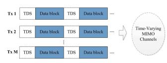
The essential thing of MIMO TDS-OFDM is guard interval. Pseudo noise sequences are utilized as guard intervals in the TDS-OFDM system. To evaluate the channel variation model, it places the assessment of channel outcomes from the PN sequences before and posterior to the data block of OFDM. The frame structure of MIMO TDS-OFDM show in Figure 1.
Figure 1. MIMO TDS-OFDM frame design
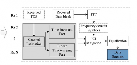
Throughout TDS-OFDM, some known sequences of reference symbols are taken as guard intervals between data to serve both channel estimation and synchronization purposes. MIMO TDS-OFDM uses the guard interval for sequences of PNs. TDS-OFDM uses the guard interval of pseudo-noise sequences which can be easily estimated. The receiver structure of MIMO TDS-OFDM for ICI suppression is show in Figure 2. The PN sequences are provided to the OFDM data block before and posterior that are used to determine the model of channel variation. In the suggested work, the standard frame structure and receiver structure intended for MIMO TDS-OFDM using the proposed ICI reduction algorithm are explained in detail.
Figure 2. MIMO TDS-OFDM receiver under ICI suppression
2.3 Cooperative communication
Here, we have a dialog about the conceivable advantages of utilizing helpful correspondence in remote correspondence systems. The remote correspondence channel experience using several marvels that lessen its solidness. At the point when the immediate transmission between the first source and goal isn't effective, other system elements can participate with the source hub to forward the information towards the goal. Henceforth, correspondence took place through various transmission ways between the source and goal hubs through the collaborating substances i.e. relay. Along these lines, numerous duplicates of transmitted data gotten by the goal hub. Goal hub in light of spatial decent variety can enhance the transmission precision by blending the information got from distinctive elements. There are numerous hubs in communicate locale of the remote correspondence medium which results in impedance to one another in their inclusion zone. With the help of cooperative communication, the transmitted power requirement at source node reduced to a level by the introduction of cooperative relay. This is because of good relay links channel condition, which significantly reduces the nosiness region.
The above Eq. (7) of received signal at the receiver can be rewritten as
$Y=\left( H+A\bar{B} \right)Z+W=\left[ H\,A \right]\left[ \begin{matrix} I \\ {\bar{B}} \\\end{matrix} \right]Z+W$ (8)
Substituting
$\hat{Z}=\left[ \begin{matrix} I \\ {\bar{B}} \\\end{matrix} \right]Z=\left[ \begin{matrix} Z \\ \bar{B}Z \\\end{matrix} \right]=\left[ \begin{matrix} Z \\ {{Z}'} \\\end{matrix} \right]$ (9)
Putting the value of Eq. (9) in Eq. (8), received signal will be,
$Y=\left[ H\,A \right]\hat{Z}+W=\left[ H\,A \right]\left[ \begin{matrix} Z \\ {{Z}'} \\\end{matrix} \right]+W$ (10)
Here,
$H=\left[\begin{array}{cccc}H_{1,1} & H_{2,1} & \dots & H_{N, 1} \\ H_{1,2} & H_{2,2} & \dots & H_{N, 2} \\ \cdot & \cdot & & \cdot \\ & \cdot & \ddots & \cdot \\ \cdot & \cdot & & \cdot \\ H_{1, M} & H_{2, M} & \dots & H_{N, M}\end{array}\right],$ (11)
$A=\left[\begin{array}{cccc}A_{1,1} & A_{2,1} & \dots & A_{N, 1} \\ A_{1,2} & A_{2,2} & \dots & A_{N, 2} \\ \cdot & \cdot & & \cdot \\ \cdot & \cdot & \ddots & \cdot \\ \cdot & \cdot & & \cdot \\ A_{1, M} & A_{2, M} & \dots & A_{N, M}\end{array}\right],$ (12)
$B=\left[ \begin{align} & B \\ & \,\,\,\,\,\,\,B \\ & \,\,\,\,\,\,\,\,\,\,\,\,\,\,\ddots \\ & \,\,\,\,\,\,\,\,\,\,\,\,\,\,\,\,\,\,\,\,\,\,\,\,B \\ \end{align} \right],$ (13)
The actual OFDM symbols in (3) formulate the $Z$ vector. Then the ${Z}'$ means? Admittedly${Z}'=\bar{B}Z$, to establish ICI, ${Z}'$ is multiplied by $A$. The formulation of $Z$ is $Z=\left\{ {{Z}_{m,k}} \right\}_{m=1,k=1}^{M,K}={{\left[ Z_{1}^{T},Z_{2}^{T},Z_{3}^{T},....,Z_{M}^{T} \right]}^{T}}$. From this ${Z}'$ is formulated as $Z^{\prime}=\left\{Z_{m, k}^{\prime}\right\}_{m=1, k=1}^{M, K}=\left[Z_{1}^{\prime T}, Z_{2}^{\prime T}, Z_{3}^{\prime T}, \ldots ., Z_{M}^{\prime T}\right]^{T}$.. Where, ${{Z}_{m,k}}-{{k}^{th}}$ subcarrier transmitted symbol. ${{{Z}'}_{m,k}}-{{k}^{th}}$ subcarrier interference (interference only on subcarrier $k$).$\bar{B}$in ${Z}'$ controls the disturbance between several subcarriers.
Hence, the channels which are invariant with time are denoted in matrix $H$. and it gives the signal transfer description without any disturbance. The channels which are variant with time are denoted in matrix $A$ and it gives the description of interference transfer itself.
Eq. (10) shows the transfer function of$2N$-transmitter, $M$-receiver MIMO-OFDM with the subcarriers $K$. In equivalent system there is no ICI interference, therefore the equalizer can be parallelized on each subcarrier.
For ${{k}^{th}}$ subcarrier,
${{\bar{Y}}_{k}}={{\left[ {{Y}_{1,k}},{{Y}_{2,k}}....,{{Y}_{M,k}} \right]}^{T}},$ (14)
${{\hat{Z}}_{k}}={{\left[ {{Z}_{1,k}},{{Z}_{2,k}}....,{{Z}_{N,k}},{{{{Z}'}}_{1,k}},{{{{Z}'}}_{2,k}}....,{{{{Z}'}}_{N,k}} \right]}^{T}},$ (15)
$\bar{H}_{k}=\left[\begin{array}{cccc}H_{1,1, k} & H_{2,1, k} & \dots & H_{N, 1, k} \\ H_{1,2, k} & H_{2,2, k} & \dots & H_{N, 2, k} \\ \cdot & \cdot && \cdot \\ \cdot & \cdot & \ddots & \cdot \\ \cdot & \cdot & & \cdot \\ H_{1, M, k} & H_{2, M, k} & \dots & H_{N, M, k}\end{array}\right]$ (16)
$\bar{A}_{k}=\left[\begin{array}{cccc}A_{1,1, k} & A_{2,1, k} & \dots & A_{N, 1, k} \\ A_{1,2, k} & A_{2,2, k} & \dots & A_{N, 2, k} \\ \cdot & \cdot & & \cdot \\ \cdot & \cdot & \ddots & \cdot \\ \cdot & \cdot & & \cdot \\ A_{1, M, k} & A_{2, M, k} & \dots & A_{N, M, k}\end{array}\right]$ (17)
And
${{\bar{Y}}_{k}}=\left[ {{{\bar{H}}}_{k}}\,{{{\bar{A}}}_{k}} \right]{{\hat{Z}}_{k}}+{{\bar{W}}_{k}},$ (18)
The above equation is the transfer expression with the transmitted symbol vector ${{\hat{Z}}_{k}}$ and received vector ${{\bar{Y}}_{k}}$ in the standard flat- fading MIMO system. Along these lines, customary OFDM equalizer with $2N$ transmitters and $M$ collectors could be utilized to even out the transmitted symbols on subcarrier $k$.
At the point when a direct MMSE (LMMSE) equalizer is utilized,
${{\hat{Z}}_{k}}\approx {{\mathbb{C}}_{{{{\hat{Z}}}_{k}}}}\left[ \begin{matrix} \bar{H}_{k}^{H} \\ \bar{A}_{k}^{H} \\\end{matrix} \right]{{\left( \left[ {{{\bar{H}}}_{k}}+{{{\bar{A}}}_{k}} \right]{{\mathbb{C}}_{{{{\hat{Z}}}_{k}}}}\left[ \begin{matrix} \bar{H}_{k}^{H} \\ \bar{A}_{k}^{H} \\\end{matrix} \right]+\delta I \right)}^{-1}}{{\bar{Y}}_{k}}$ (19)
The vector $\hat{Z}$ consist of the evaluation of the transmitted symbols. To achieve better evaluation presentation, $Z$ is evaluated as
$\ddot{Z}=E\hat{Z}={{\mathbb{C}}_{Z\hat{Z}}}\mathbb{C}_{\hat{Z}\hat{Z}}^{-1}\hat{Z}=\left[ I\,\,\,{{{\bar{B}}}^{H}} \right]{{\left[ \begin{matrix} I & {{{\bar{B}}}^{H}} \\ {\bar{B}} & \bar{B}{{{\bar{B}}}^{H}} \\\end{matrix} \right]}^{-1}}\hat{Z}.$ (20)
With the matrix
$E={{\mathbb{C}}_{Z\hat{Z}}}\mathbb{C}_{\hat{Z}\hat{Z}}^{-1}=\left[ I\,\,\,{{{\bar{B}}}^{H}} \right]{{\left[ \begin{matrix} I & {{{\bar{B}}}^{H}} \\ {\bar{B}} & \bar{B}{{{\bar{B}}}^{H}} \\\end{matrix} \right]}^{-1}}.$ (21)
Even though transposition of a broad matrix is involved, the $E$ is a precalculated matrix and acts like a predesigned linear filter then the determination of matrix $E$ is defined only by$N$, $M$ and $k$, therefore it’s irrelevant to channel realization. The complexity is restricted to filtering itself. ${{\mathbb{C}}_{{{{\hat{Z}}}_{k}}}}$ is covariance matrix of the transmitted symbol vector. The matrix is a $2N\times 2N$ sub matrix containing of the components at the ${{k}^{th}}$, $K+{{k}^{th}}$ … and $(2N-1)K+{{k}^{th}}$ rows and columns of the matrix ${{\mathbb{C}}_{\hat{Z}\hat{Z}}}$ that’s why the transposition of ${{\mathbb{C}}_{{{{\hat{Z}}}_{k}}}}$ can again pre calculated.
Correlation between the LMMSE equalizer in MIMO-OFDM again performances subcarrier by subcarrier. The only dissimilar is that the subsystem transfer function in each subcarrier does not contain the time varying matrix ${{\bar{A}}_{k}}$,
${{\bar{Y}}_{k}}={{\bar{H}}_{k}}{{\bar{Z}}_{k}}+{{\bar{W}}_{k}}.$ (22)
Then the demodulation in LTI channels is
${{\bar{Z}}_{k}}\approx {{\mathbb{C}}_{{{{\bar{Z}}}_{k}}}}\bar{H}_{k}^{H}{{\left( \bar{H}_{k}^{H}{{\mathbb{C}}_{{{{\bar{Z}}}_{k}}}}\bar{H}_{k}^{H}+\delta I \right)}^{-1}}{{\bar{Y}}_{k}}.$ (23)
For equalization under the assumption of LTI channels, several computations occur when multiplication of matrixes for each subcarrier is performed as in (23). The complexity for both algorithms is linear to the number of subcarriers and cubic to the number of receivers when the number of transmitters and receivers is in the same order. But when compared with the equalizer in LTI channels, the proposed algorithm has remained fairly small in complexity. Table 1 shows the complexity of different equalizers. Our proposed algorithm is having less complexity in comparison to other algorithms.
Table 1. Complexity of different equalizers
|
Technique |
Complexity |
|
LMMSE in LTI1 |
$O\,\left( K\left( {{M}^{3}}+N{{M}^{2}}+NM+M\log \left( K \right) \right) \right)$ |
|
Proposed in LTV2 |
$O\,\left( K\left( {{M}^{3}}+2N{{M}^{2}}+2NM+2{{N}^{2}}+M\log \left( K \right) \right) \right)$ |
|
Original in LTV3 |
$O\,\left( {{K}^{3}}\left( {{M}^{3}}+N{{M}^{2}}+NM \right)+MK\log \left( K \right) \right)$ |
4.1 Stanford University Interim (SUI) channel model
This is a set of 6 channel models representing three terrain types and a variety of Doppler spreads, delay spread and line-of-sight/non-line-of-sight conditions that are typical of the continental US.
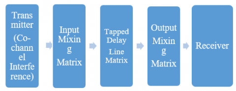
Figure 3 below shows the Basic structure of Stanford University Interim (SUI) channel model. It has mainly three blocks namely input mixing matrix, tapped delay line matrix and output mixing matrix.
Figure 3. Basic Structure of SUI channel models
4.1.1 Input mixing matrix
This part models correlation between input signals if multiple transmitting antennas are used.
4.1.2 Tapped delay line matrix
This part models the multipath fading of the channel. The multipath fading is modelled as a tapped delay line with 3 taps with non-uniform delays. The gain associated with each tap is characterized by a distribution (Rician with a $\delta $ -factor > 0, or Raleigh with $\delta $ -factor=0) and the maximum Doppler frequency.
4.1.3 Output mixing matrix
This part models the correlation between output signals if multiple receiving antennas are used. Using the above general structure of the SUI Channel and assuming the following scenario, six SUI channels are constructed which are representative of the real channels.
Simulations are carried out to evaluate the efficiency of the methodology proposed. The traditional equalizer is also evaluated for comparison under the assumption of invariant channel time.
Then the quantity of transmitters has been 2, as well as the number of beneficiaries is 4, 8, 12. This framework takes TDS-OFDM in MIMO construction through PN-extensive with rotate (PN-ER) [3], when time-space arrangements to helpfully access the MIMO channels. Then the data transmission is 1 MHz, as well as framework, have $K=1024$ subcarriers, hence every subcarrier bears around 1 kHz on transfer speed. A data bit is autonomously as well as uncoded QPSK/16QAM tweaked to every Tx. This reenactment takes MIMO channel postpones profiles and changes the Doppler recurrence of the Rayleigh blurring channels to test the execution of the proposed calculation. The most extreme Doppler move on this recreation to be 100 Hz, or identically Doppler factor is 0.1. In the proposed system, the channel experience long multipath delay and is very recurrence specific.
5.1 Experimental result for Channel-A
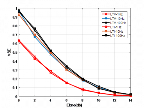
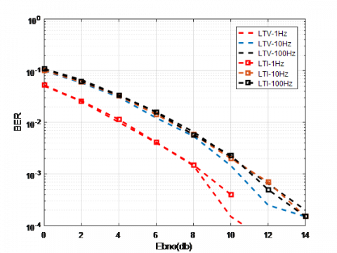
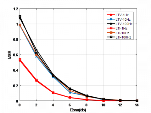
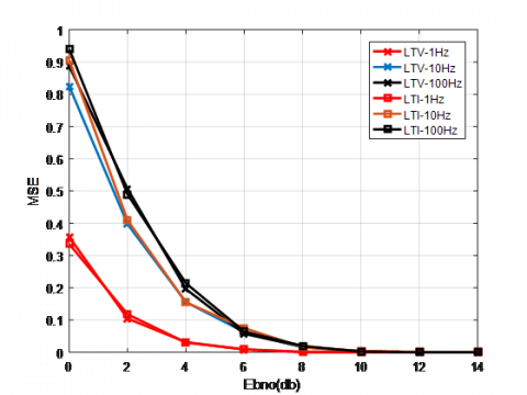
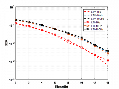
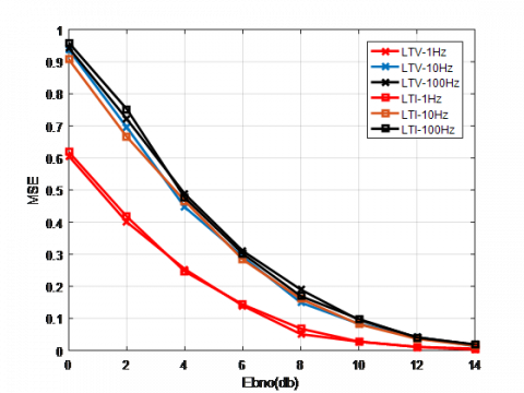
To show the execution of the proposed calculation, we first analyze the three calculations within the sight of two distinctive channels. The principal ("Channel A") is the channel with the Doppler range following a Gaussian dispersion. The focused Doppler recurrence is $0.9{{f}_{D}}$, and the sigma of the Gaussian dispersion is $0.001{{f}_{D}}$, where ${{f}_{D}}$ is the greatest Doppler move. Accordingly, this channel is A channel Figure 4, Figure 6, Figure 8 show BER of QPSK modulated signal when $M=4,8,12$. Figure 5, Figure 7, Figure 9 show MSE of QPSK modulated signal when $M=4,8,12$. Evening out BER execution of 16QAM when $M=4,8,12$ to have almost predominant Doppler move. Then another ("Channel B"), this Doppler extends any ways pursues Jakes Doppler range with most extreme Doppler move${{f}_{D}}$. So Channel B has a more complex time-fluctuating element than Channel A.
Figure 4. BER performance for both LTI and LTV channels having two transmitters and 4 receivers, modulation is QPSK
Figure 5. MSE performance for both LTI and LTV channels having two transmitters and 4 receivers, modulation is QPSK
Figure 6. BER performance for both LTI and LTV channels having two transmitters and 8 receivers, modulation is QPSK
Figure 7. MSE performance for both LTI and LTV channels having two transmitters and 8 receivers, modulation is QPSK
Figure 8. BER performance for both LTI and LTV channels having two transmitters and 8 receivers, modulation is QPSK
Figure 9. MSE performance for both LTI and LTV channels having two transmitters and 8 receivers, modulation is QPSK
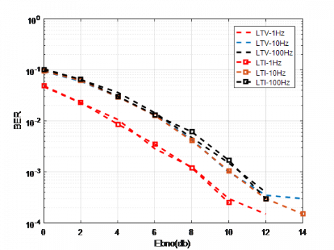
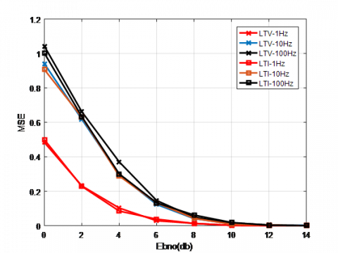
5.2 Experimental result for Channel-B
In below Figure 10 to Figure 15 show MSE and uncodify BER execution on Channel B with QPSK modulation. Here we have taken three different frequency${{f}_{D}}=1Hz,\,50Hz$ and$100Hz$. A typical overwhelming Doppler move as mainly achieve through different time-channels, this technique on [4] as around 0.3 dB character SNR improvement more than these “linear time independent” equalizer while BER is somewhere in the range of 10−3 and 10−2,because Channel B nearly complies with its channel blurring suspicion. Not with standing, in Channel B, " linear time independent" perform superior to than calculation on [4] in light of the fact that distinctive channel ways may have diverse time-changing profiles consequently disregard the supposition of the calculation on [4]. The equally Channel A and Channel B, the expected calculation as demonstrated the greatest MSE and BER execution among the three.
Figure 10. BER performance for both LTI and LTV channels having two transmitters and four receivers, modulation is QPSK
Figure 11. MSE performance for both LTI and LTV channels having two transmitters and four receivers, modulation is QPSK
Figure 12. BER performance for both LTI and LTV channels having two transmitters and 8 receivers, modulation is QPSK
Figure 13. MSE performance for both LTI and LTV channels having two transmitters and 8 receivers, modulation is QPSK
Figure 14. BER performance for both LTI and LTV channels having two transmitters and 12 receivers, modulation is QPSK
Figure 15. MSE performanc for both LTI and LTV channels having two transmitters and 12 receivers, modulation is QPSK
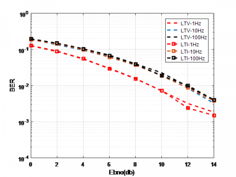
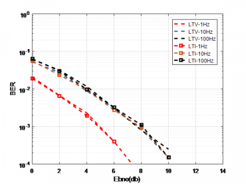
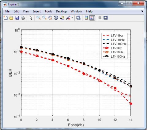
The below Figure 16 shows the extension result having better BER performance in comparison to previous results. The different between BER for LTI at ${{f}_{D}}=1Hz\,and\,100Hz$is very small in comparison to previous one at $0.2dB$SNR. BER performance of the three methodologies is compared to QPSK modulation if ${{f}_{D}}=1Hz,\,50Hz\,and\,100Hz$. We can see that the BER of both methods increases as the maximum Doppler shift decreases, suggesting a more extreme inter-carrier interference effect increased with the maximum Doppler shift. When more receivers are used the BER gets smaller, which is the product of more range gain with much more receiving units. At the same time, the suggested method always has a lower MSE than that of the traditional equalizer when ${{f}_{D}}=1Hz,\,50Hz\,and\,100Hz$. Also, the suggested method outperforms the LTI equalizer whenever the Doppler frequency is ${{f}_{D}}=1Hz,\,50Hz\,and\,100Hz$.
Figure 16. BER performance for SUI channels
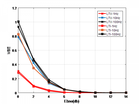
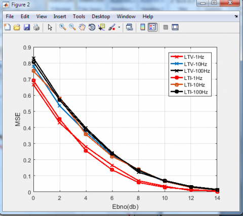
Figure 17. MSE performance for SUI channels
MSE performance of the three methodologies is being analysed to QPSK modulation for ${{f}_{D}}=1Hz,\,50Hz\,and\,100Hz$. The below Figure 17 shows the extension result having better MSE performance in comparison to previous results at the high value of SNR. As the SNR increases the difference between MSE of LTV at two different frequencies decreases. The difference between MSE for LTI at ${{f}_{D}}=1Hz\,and\,100Hz$is very small in comparison to the previous one at $0.3dB$SNR. We have noticed that the MSE of both methods increases as the maximum Doppler shift decreases, suggesting a more extreme inter-carrier interference effect increased with the maximum Doppler shift. At the same time, the suggested method always has a lower MSE than that of the traditional equalizer when ${{f}_{D}}=1Hz,\,50Hz\,and\,100Hz$. It has been noticed that at high SNR of $14dB$ MSE between LTI or LTV at different frequency is negligible.
In this article, a low-complexity ICI reduction methodology is implemented in MIMO-OFDM. The methodology uses the ICI contribution framework in linear time and maintains low complexity in various channels. Simulations have shown that the suggested solution outperforms conventional equalization under LTI assumption with a gain of up to $2dB$ SNR when the comparative Doppler factor is 0.1. The methodology is an extension of MIMO from the original SISO algorithms in [3]-[5 ]. Such methodology all use a linear time variance model to achieve ICI compensation in OFDM systems at low complexity. Future work on a similar or extended methodology based on this work, such as equalization with the cancelation of iterative interference and turbo equalization with measurement of soft information is possible.
[1] Dai, L., Wang, Z., Yang, Z. (2012). Next-generation digital television terrestrial broadcasting systems: Key technologies and research trends. IEEE Commun. Mag., 50(6): 150-158. https://doi.org/10.1109/MCOM.2012.6211500
[2] Fu, J., Pan, C.Y., Yang, X.Z., Yang, L. (2005). Low-complexity equalization for TDS-OFDM systems over doubly selective channels. IEEE Trans. Broadcast., 51(3): 401-407. https://doi.org/10.1109/TBC.2005.852249
[3] Armstrong, J. (1999). Analysis of new and existing methods of reducing Intercarrier interference due to carrier frequency offset in OFDM. IEEE Trans. Commun., 47(3): 365-369. https://doi.org/10.1109/26.752816
[4] Wu, H.C. (2006). Analysis and characterization of Intercarrier and interblock interferences for wireless mobile OFDM systems. IEEE Trans. Broadcast., 52(2): 203-210. https://doi.org/10.1109/TBC.2006.872989
[5] Li, B., Huang, J., Zhou, S., Ball, K., Stojanovic, M., Freitage, L., Willett, P. (2009). MIMO-OFDM for high-rate underwater acoustic communications. IEEE J. Ocean. Eng., 34(4): 634-644. https://doi.org/10.1109/JOE.2009.2032005
[6] Shankar, R., Kumar, I., Mishra R.K. (2019). Outage probability analysis of MIMO-OSTBC relaying network over Nakagami-m fading channel conditions. Traitement du Signal, 36(1): 59-64. https://doi.org/10.18280/ts.360108
[7] Huang, J., Zhou, S., Wang, Z. (2013). Performance results of two iterative receivers for distributed MIMO OFDM with large Doppler deviations. IEEE J. Ocean. Eng., 38(2): 347-357. https://doi.org/10.1109/JOE.2012.2223991
[8] Dai, L., Wang, Z., Wang, J., Yang, Z. (2013). Joint time-frequency channel estimation for time domain synchronous OFDM systems. IEEE Trans. Broadcast., 59(1): 168-173. https://doi.org/10.1109/TBC.2012.2219231
[9] Kumar, I., Sachan, V., Shankar, R., Mishra, R.K. (2018). An investigation of wireless S-DF hybrid satellite terrestrial relaying network over time selective fading channel. Traitement du Signal, 35(2): 103-120. https://doi.org/10.3166/ts.35.103-120
[10] Sachan, V., Shankar, R., Kumar, I., Mishra, R.K. (2019). Performance analysis of SM-MIMO system employing binary PSK and M’ary PSK techniques over different fading channels. Procedia Computer Science, 152: 323-332. https://doi.org/10.1016/j.procs.2019.05.010
[11] Shankar, R., Kumar, I., Kumari, A., Pandey, K.N., Mishra, R.K. (2019). Pairwise error probability analysis and optimal power allocation for selective decode-forward protocol over Nakagami-m fading channels. International Conference on Algorithms, Methodology, Models and Applications in Emerging Technologies (ICAMMAET), Chennai, India, pp. 1-6. https://doi.org/10.1109/ICAMMAET.2017.8186700
[12] Shankar, R., Kumar, I., Mishra, R.K. (2019). Pairwise error probability analysis of dual hop relaying network over time selective Nakagami-m fading channel with imperfect CSI and node mobility. Traitement du Signal, 36(3): 281-295. https://doi.org/10.18280/ts.360312
[13] Du, X., Tadrous, J., Sabharwal, A. (2016). Sequential beamforming for multiuser MIMO with full-duplex training. IEEE Trans. Wireless Commun., 15(12): 8551-8564. https://doi.org/10.1109/TWC.2016.2616338
[14] Sachan, V., Kumar, I., Shankar, R., Mishra, R. K. (2018). Analysis of transmit antenna selection based selective decode forward cooperative communication protocol. Traitement du Signal, 35(1): 47-60. https://doi.org/10.3166/ts.35.47-60
[15] Weingarten, H., Steinberg, Y., Shamai, S. (2006). The capacity region of the Gaussian multiple-input multiple output broadcast channel. IEEE Trans. Inf. Theory, 52(9): 3936-3964. https://doi.org/10.1109/TIT.2006.880064