Suman Machavarapu* | Mannam Venu Gopala Rao | Pulipaka Venkata Ramana Rao
OPEN ACCESS
A novel Extreme learning Machine (ELM) algorithm based tuning of the parameters of the SVC FACTS controller was implemented in order to control voltage at various buses over a wide range. The ELM algorithm is a non-iterative method which forecasts the parameters of SVC FACTS controller quickly and effectively while Back Propagation Neural Network (BPNN) algorithm is an iterative method which takes a long time for training as well prediction of parameters. The load perturbation is one of the nonlinear disturbances which is considered to investigate the operational capability of the control methodology. Standard IEEE 5 and 30 bus systems are considered as test systems and operation of two models of SVC observed with the BPNN and ELM controllers. The weakest bus is identified using L-Index method which is the optimal location of the SVC FACTS. Results show that the novel ELM method expeditiously and efficiently tunes the parameters of the SVC FACTS controller online such that the voltage regulated to desired value when there is a perturbation in load.
voltage stability, SVC FACTS controller, susceptance model, firing angle model, BPNN algorithm, ELM algorithm
The voltage stability improvement of the interconnected power system drawn significant importance over a few decades [1]. The key concern of the modern power systems is to transmit and supply the generated power effectively at high power quality. In practical operation of power systems many unwanted disturbances such as load variations, faults, unmodeled dynamics and, parametric uncertainties cause power quality issues. In general mismatch between reactive power generation and reactive power requirement leads to variation in voltage.
In modern interconnected system, heavy loading leads to voltage dip which will affect the security and reliability of the system. The Load on the power system is continuously varies with respect to time so the reactive power, requirement also varying which leads to variation in voltage which is undesirable. The reactive power requirement may be supplied with local support thereby voltage can be maintained within the limits. Static VAR compensator is a power electronic based controller which can absorb or generate reactive power [2]. It can be used for voltage support, power oscillation damping, and stability improvement.
Rahman et al. [3] proposed PID controller based SVC to enhance the voltage stability. The PID controller parameters are tuned using the Nichols- Ziegler method. A single machine connected to the infinite bus is considered as a test system and the operational capability of the proposed controller is observed with L-G and L-L fault.
A Static VAR Compensator was developed by Priyadhershni et al. [4] to enhance the voltage profile of the standard IEEE 5 and 14 bus systems. In this paper SVC FACTS controller, the operational capability is observed with a perturbation in load. It was clearly observed that the proposed controller can effectively compensate the voltage variations caused by the various disturbances. The modern Static VAR System (SVS) designed by Pouyan et al. [5] SVSs was the combination of the capacitors with automatic switching and Static VAR Compensator. PG&E Bay area in San Francisco is considered as a test system. Two different areas are equipped with SVS controllers to enhance the dynamic and transient stability.
Chang [6] optimally placed the SVC FACTS controller such that the loading margin was improved to required level and minimize the cost of expansion. Here a multi objective function is minimised to identify the optimal placement and cost of the controller. Model analysis is used to identify which bus require SVC installation. The implemented technique is validated on the IEEE 24 bus power system.
Rahman et al. [7] developed a new SVC strategy which will operate in coordination with ULTC. SVC is a fast acting device where as ULTC is a slow acting control. Whenever there is a deviation in voltage SVC acts first and its maximum power limit violated it does not have control over active power and will act as a normal capacitor bank. Coordination operation was developed between SVC controller and ULTC.
Hari Krishna et al. [8] designed the ANN based SVC FACTS controller which not only improves the voltage profile but also damp the rotor low frequency oscillations. The data obtained conventional controllers neural network will be trained. Simulation results shows that ANN based SVC damping controller provides better damping compared to the PID based SVC damping controller.
Abood [9] modelled SVC controller to improve the voltage stability. Neuro-PID controller is designed to enhance the response. The output of the developed controller is compared with the conventional PID based SVC controller output. The Neuro-PID SVC controller enhances the voltage at buses better than PID based SVC controller.
In this paper SVC FACTS controller is included in Newton Raphson load flow method, optimal siting of FACTS controller is determined using the L-index method for IEEE 5 and 30 bus systems. Later BPNN and ELM algorithms are used to train the ANN for the prediction of parameters of SVC FACTS controller. The main drawbacks of the BPNN are network paralysis, local minima and slow convergence because it is using gradient descent method. The proposed method predicts the parameters quickly and effectively and eliminates the disadvantages in the BPNN.
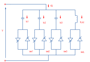
SVC [10] is the combination of Thyristor Controlled Reactor (TCR) and Thyristor Switched Capacitor (TSC) which is utilized for the dynamic compensation of transmission lines. It will likewise enhance the working adaptability and minimizes the losses in the power system. A basic SVC structure is as shown in Figure 1 which consists of three TSCs and one TCR. The quantity of TSCs required is principally relies upon working voltage, required most extreme power yield and current rating of the thyristor valves Inductive rating might be stretched out by including the number of TCRs dependent on the necessity. If the voltage is below the reference value TSC will act and create the required reactive power with the end goal that voltage takes back to reference level and if the voltage is more than reference value TCR will act.
Figure 1. SVC FACTS controller
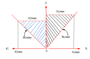
Figure 2. V-I characteristics of SVC FACTS controller
The Volt-Amp characteristics of the SVC FACTS controller are as shown in Figure 2. The SVC can also be used to enhance the voltage profile at the midpoint and at the end of the lines, Improvement of dynamic and transient stability and Power oscillation damping.
2.1 Modelling of static VAR compensator
SVC can be mathematically modelled using susceptance and firing angle model as given in 2.1.1 and 2.1.2.
2.1.1 Susceptance method
The equivalent circuit is used to obtain the SVC FACTS controller power equations and the equations required by NR method [11]. In this method susceptance is varied until the voltage return back to a reference level.
The current drawn by the SVC is given at bus k is given as
${{I}_{SV{{C}^{.}}}}=j*{{B}_{SVC}}*{{V}_{k}}$ (1)
The reactive power injected at bus k.
${{Q}^{.}}_{SVC}={{Q}_{k}}=-V_{k}^{2}*{{B}_{SVC}}^{.}$ (2)
The linearized equation is given by the following Eq. 3
${{\left[ \begin{matrix} \Delta {{P}_{{{k}^{.}}}} \\ \Delta {{Q}_{{{k}^{.}}}} \\\end{matrix} \right]}^{(i)}}={{\left[ \begin{matrix} {{0}^{.}} & {{0}^{.}} \\ {{0}^{.}} & {{Q}_{{{k}^{.}}}} \\\end{matrix} \right]}^{(i)}}{{\left[ \begin{matrix} \Delta {{\theta }_{{{k}^{.}}}} \\ {}^{\Delta {{B}_{SVC}}^{.}}/{}_{{{B}_{SVC}}^{.}} \\\end{matrix} \right]}^{(i)}}$ (3)
2.1.2 Firing angle method
In firing angle method $B_{S V C}$ is given by Eq. 4
$\begin{array}{l}{\mathrm{B}_{\mathrm{svc}}=\mathrm{B}_{\mathrm{C}}-\mathrm{B}_{\mathrm{TCR}}=\frac{1}{X_{C} * X_{L}}\left\{X_{L}-\frac{X_{C}}{\prod} *[2 *(\Pi-\alpha)+\sin 2 \alpha]\right\}} \\ {X_{L}=\omega^{*} L} \\ {X_{C}=\frac{1}{\omega^{*} C}}\end{array}$ (4)
In firing angle method reactive power generated at bus k is given as Eq. 5
$Q_{k}=-\frac{V_{k}^{2}}{X_{C} * X_{L}}\left\{X_{L}-\frac{X_{C}}{\Pi} *[2 *(\Pi-\alpha)+\sin 2 \alpha]\right\}$ (5)
From Eq. 5, the linearised SVC equation can be written as Eq. 6
$\left[\begin{array}{c}{\Delta P_{k}} \\ {\Delta Q_{k}}\end{array}\right]=\left[\begin{array}{cc}{0} & {0} \\ {0} & {\frac{2 * V^{2}}{\Pi^{*} X_{L}}[\cos (2 \alpha)-1]}\end{array}\right]\left[\begin{array}{c}{\Delta \theta_{k}} \\ {\Delta \alpha}\end{array}\right]$ (6)
Kessel [12] developed L-index which is a simple method and has been used as the indicator of the voltage stability of the transmission line. It will give online monitoring of voltage sensitivity at all load buses with sufficient accuracy. It can be used for both static and dynamic situations of the power system. It can also use to determine the weak points on the system, stability margin and different parameters of the voltage stability. Various algorithms developed to determine voltage sensitivity using static approach is laborious and does not provide voltage sensitivity in a dynamic way. L-Index changes somewhere in the range of 0 and 1 [13]. If it approaches to 0 at a particular bus, the bus is secure bus or if it approaches to 1, the particular bus is said to be the weak bus and is the optimal siting of the SVC FACTS controller. Let us consider a general system having number of buses out of which there is αG number of generator buses and αL number of load buses. The L-index value at the Jth bus can be calculated as given in Eq. 7.
${{L}_{J}}=\left| {{L}_{J}} \right|=\left| 1-\frac{\sum\limits_{I=1}^{{{\alpha }_{G}}}{{{C}_{IJ}}{{V}_{J}}}}{{{V}_{J}}} \right|$ (7)
VJ= Complex voltage at Load J.
CIJ=Elements of matrix C which can be determined using the Eq. 8.
$\left[ C \right]=-{{\left[ {{Y}_{ll}} \right]}^{-1}}\left[ {{Y}_{\lg }} \right]$ (8)
Sub matrices of YBUS matrix are [Yll ] and [Ylg] and it can be found using Eq. 9.
$\left[ \begin{matrix} I{}_{l} \\ {{I}_{g}} \\\end{matrix} \right]=\left[ \begin{matrix} {{Y}_{ll}} & {{Y}_{\lg }} \\ {{Y}_{gl}} & {{Y}_{gg}} \\\end{matrix} \right]\left| \begin{matrix} {{V}_{l}} \\ {{V}_{g}} \\\end{matrix} \right|$ (9)
ANNs are developed to impersonate the characteristics of the human brain. ANN is a blend of different Artificial Neurons. A single neuron is a processing unit and like a summing unit. At each neuron the weighted sum is calculated and the output is determined by processing through activation function. The ANN has been extensively used for massive parallelism, fault tolerance distributed representation, generalization ability, adaptively, learning ability, inherent contextual information processing and Low energy consumption. Artificial Neural Networks also used for forecasting of some parameters or controlling of some other parameters. Most of the applications use MNNs rather than single layer Neural networks which will be trained using BPNN.
4.1 Back propagation algorithm
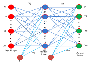
The architecture of MNN is as given in Figure 3 [14, 15]. It has an input, hidden and output layers with n,p and m number of neurons.
The input vector X is applied to neurons in the input layer and the activation values at the hidden layer can be calculated. The activation value of the jth neuron is given by Eq. 10.
${{Z}_{-inj}}=Voj+\sum\limits_{i=1}^{n}{({{X}_{i}}*{{V}_{ij}}})$ (10)
The output of the jth hidden neuron can be calculated using sigmoidal activation function as given in Eq. 11.
$Z_{j}=f\left(Z_{\text {-inj }}\right)=\frac{1}{1+e^{Z_{-i n j}}}$ (11)
The hidden layer neurons output will be the inputs for each neuron in the output layer. The activation function at the kth neuron can be calculated using Eq. 12.
${{Y}_{-ink}}^{.}={{W}_{o{{k}^{.}}}}+{{\sum\limits_{j=1}^{p}{({{Z}_{j}}^{.}*{{W}_{jk}}}}^{.}})$ (12)
The response of the neuron in the kth output layer can be determined using sigmoidal activation function as given in Eq. 13.
Yk=f(Y-ink) = $\frac{1}{1+{{e}^{{{Y}_{-ink}}}}}$ (13)
Figure 3. Multi layer Neural Network (MNN)
The actual output of each neuron is compared with the expected output and squared error is determined. The weights are adjusted to decrease the squared error. Once outputs of the neurons in the output layer calculated, the error is calculated and the weights are adjusted to minimize the error. The updation of the weights are given as follows.
The weights between the output and hidden layer, bias neuron can be updated as follows.
Wjk.(new)=Wjk.(old)+ ΔWjk.,
Wok.(new)=Wok.(old)+ ΔWok (14)
where, ΔWjk= $\eta *\frac{\partial E}{\partial {{W}_{jk}}}$ = $\eta \text{*}{{\delta }_{\text{k}}}\text{*}{{\text{Z}}_{\text{j}}}$
ΔWok= $\eta *\frac{\partial E}{\partial {{W}_{ok}}}$ = $\eta $ * $\delta_{\mathrm{k}}$ (15)
The weights between the hidden and input layer, bias neuron will be updated as follows.
Vij (new)=Vij.(old)+ΔVij
Voj.(new) =Voj (old) + ΔVoj
where,
ΔVij= $\eta $ * δj*Xi
ΔVok=alpha*δi (16)
4.1.1 Methodology
BPNN is a procedural method for training MNNs. It is a multilayer feed forward network using extended gradient-descent based method for training which is popularly known as back propagation rule. It is a computationally efficient method for optimizing the weights in a feed-forward network. In this derivation of the squared error with respect to the weights is calculated and the weights are changed to minimize the squared error. So, the continuous activation functions are used which are differentiable. Sigmoidal activation function is mainly used which is the continuous approximation of the step function. The network is trained by supervised learning method. The aim of this algorithm is to train the multi layer neural network to achieve a balance between the output and expected output and ability to respond correctly to the input patterns that is used for training and the ability to provide better responses to the input that are similar. The BPNN Algorithm is as given below.
Step 1: Initialize all weights to random values
Step 2: Apply the deviation in voltage as input to the BPNN.
Step 3: Calculate the outputs of the hidden and output layers in forward pass.
Step 4: Determine the squared error which is to be minimised for better training.
Step 5: Update the weights between output and hidden, hidden and input layers in the backward process.
Step 6: Repeat the pocedure till the squared error is blow 0.001.
Several drawbacks in the Back propagation algorithm are
4.2 Extreme learning machine algorithm
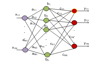
The bottlenecks in the BPNN Algorithm, ELM is proposed [16]. ELM network is a single hidden layer feed forward NN as shown in Figure. In this network, input weights and biases are initialized randomly and the output weights are calculated analytically.
Mathematically, let (xi, yi)i=1N are the patterns formulated to train ELM network. Where xi is input variable contains p number of attributes and yi is output variable contains q number of attributes. The mathematical model of ELM with h number of neurons and with activation function G(.) is expressed as:
$Y({{x}_{k}})=\sum\limits_{i=1}^{h}{{{C}_{i}}}G({{x}_{i}}.{{a}_{k}}+{{b}_{i}})\,\,\,\,,k=1,2,....N$ (17)
where, c matrix is output weight matrix, a is input weight matrix and b is the bias matrix.
The ELM network is depicted as shown in Figure 4.
The Eq. (17) can be written in matrix notation as:
$\mathrm{G} \mathrm{C}=\mathrm{Y}$ (18)
where, G is matrix of outputs of hidden layer and Y is output
matrix of ELM n $\left[ \begin{matrix} g(a1*x1+b1) & \circ & \circ & g(an*x1+bn) \\ \circ & \circ & \circ & \circ \\ \circ & \circ & \circ & \circ \\ g(a1*xn+b1) & {} & {} & g(an*xn+bn \\\end{matrix} \right]$ (19)
$\beta =\left[ \begin{matrix} C_{1}^{T} \\ \circ \\ \circ \\ C_{n}^{T} \\\end{matrix} \right]$ $Y=\left[ \begin{matrix} y_{1}^{T} \\ \circ \\ \circ \\ y_{n}^{T} \\\end{matrix} \right]$
This can be compared similar to the cost function minimization in gradient based back propagation algorithm.
${{F}_{BP}}=\sum\limits_{i=1}^{N}{\left[ \sum\limits_{j=1}^{h}{{{\beta }_{j}}}G({{x}_{i}}.{{a}_{j}}+{{b}_{i}})-{{y}_{i}} \right]}$ (20)
For randomly assigned input weights and biases the output weight matrix elements are calculated as:
$C={{G}^{+}}Y$ (21)
where, G+ is the Moore – Penrose inverse of G matrix, which is evaluated from Singular value decomposition.
Figure 4. Layout of single hidden layer ELM network
4.2.1 Methodology
In this work, the voltage variation fed as input to the ELM network and the corresponding firing angle and susceptance is forecasted for SVC FACTS controller to bring back the voltage to the actual reference value. The implementation of ELM is given in following steps
Step 1: The voltage variation at the busses is given as input for ELM network
Step 2: Input weights and biases are generated randomly and the output weights are calculated analytically.
Step 3: With the obtained output weights, the output firing angle or susceptance will be predicted.
Step 4: Using the updated firing angle or susceptance the voltage profile of the system is improved.
The ELM is having diverse assets when compared to the classical learning techniques in terms of high speed learning, greater generalization performance, uses non differential activation function, not suffered with over fitting, local minima and imprecision in learning.
For 5-bus and 30-bus L-index values are calculated. In 5-bus system, it was observed that 5th bus is having highest L- index value i.e. 0.0774 which is the critical bus. In the 30-bus system, there is high L-index value, i.e. 0.142 at 30th bus, so it is the optimal location of the SVC FACTS controller. L-index values for 5-bus and 30-bus are as given in Table 1 and Table 2 respectively.
Table 1. L-Index values at load buses of 5-bus system
|
Bus No. |
L-Index |
|
5 |
0.0774 |
|
3 |
0.064 |
|
4 |
0.0397 |
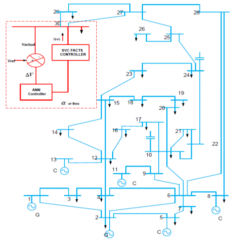
The 30-bus power system with ANN based SVC FACTS controller is as shown in Figure 5. Whenever there is a change in load demand there will be voltage drop which is sensed by the ANN controller and generate necessary signals to an SVC FACTS controller such that voltage brings back to tolerance level.
Table 2. L-Index values at load buses of 30-bus system
|
Bus No. |
L-index |
Bus No. |
L-index |
|
30 |
0.142 |
23 |
0.0611 |
|
3 |
0.1252 |
21 |
0.0577 |
|
4 |
0.1038 |
26 |
0.0577 |
|
29 |
0.0925 |
10 |
0.0568 |
|
6 |
0.091 |
22 |
0.0564 |
|
7 |
0.0889 |
14 |
0.0546 |
|
19 |
0.0718 |
17 |
0.0533 |
|
18 |
0.0677 |
16 |
0.0499 |
|
15 |
0.0671 |
25 |
0.0461 |
|
20 |
0.0664 |
27 |
0.0424 |
|
28 |
0.0638 |
12 |
0.0384 |
|
24 |
0.0614 |
9 |
0.0347 |
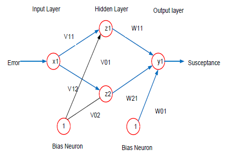
Figure 6. Neural network to predict susceptance
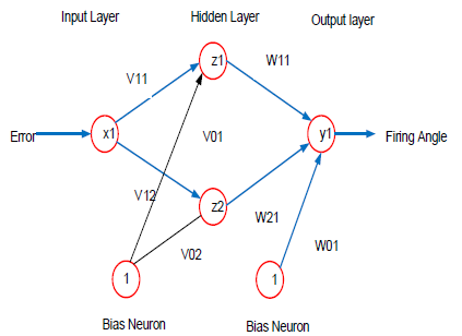
Figure 7. Neural network to predict firing angle
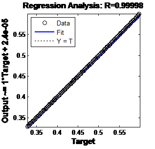
Figure 8. 5-bus BPNN susceptance method
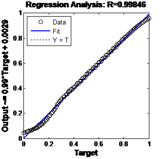
Figure 9. 5-bus ELM susceptance method
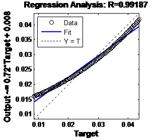
Figure 10. 5-bus BPNN firing angle method
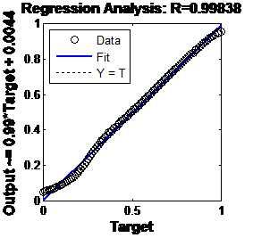
Figure 11. 5-bus ELM firing angle method
Figure 12. 30-bus ANN susceptance method
Figure 13. 30-bus ELM susceptance method
Figure 14. 5-bus BPNN firing angle method
Figure 15. 30-bus ELM firing angle method
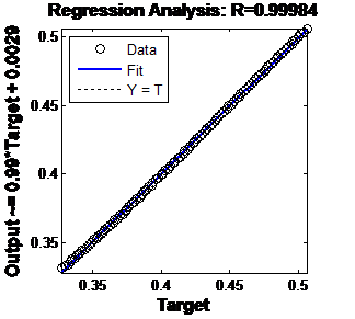
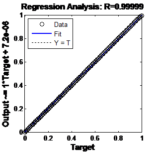
The Neural network designs for this particular problem is as given in Figures 6 & 7 for the two models considered. The regression plots which indicates the effectiveness of the training for back propagation algorithm is given as in Figures 8, 9, 10 & 11.
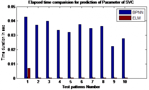
The BPNN is an iterative method and the ELM is a non-iterative method. So, the ELM method training is very low compared to BPNN. Approximately ELM is more than 1000 time faster compared to BPNN. The training time of BPNN is very high when compared to the ELM. The training times of both the methods are as given in Table 3.
The voltage improvement without and with BPNN, ELM at different loads tabulated in Table 4, Table 5, Table 6 and Table 7. From the tables it was clearly observed that the ELM is outperforming the BPNN in terms of accuracy as well timing. The elapsed time taken by BPNN and ELM is tabulated and clearly indicates after training ELM predict parameters of the SVC FACTS controller quickly compared to the BPNN. The deviation in voltage should bring back to 1 p.u using the two intelligent methods. The effectiveness of the BPNN and ELM are as shown in Figure 12, Figure 13, Figure 14 and Figure 15 (The statement will be below Table 3).
Table 3. Training times of the BPNN and ELM methods
|
S.No |
Method |
Training Time(sec) |
|
|
BPNN |
ELM |
||
|
1 |
5-bus susceptance |
102.061 |
0.01355 |
|
2 |
5-bus firing angle |
847.897 |
00112 |
|
3 |
30-bus susceptance |
1016.194 |
0.0146 |
|
4 |
30-bus firing angle |
635.8188 |
0.0112 |
Table 4. Comparison between ELM and BPNN methods with 5-bus SVC susceptance model
|
S.No |
%of change in load |
Voltage at bus-5 without SVC |
Bsvc Predicted |
Elapsed Time |
Voltage at bus-5 with SVC |
|||
|
BPNN |
ELM |
BPNN |
ELM |
BPNN |
ELM |
|||
|
1 |
5 |
0.9694 |
0.3479 |
0.3469 |
0.042848 |
0.006977 |
1.0267 |
1.0001 |
|
2 |
10 |
0.9679 |
0.3636 |
0.363 |
0.037191 |
0.000316 |
1.0001 |
1.0000 |
|
3 |
15 |
0.9663 |
0.3805 |
0.3803 |
0.039792 |
0.000245 |
1 |
1.0000 |
|
4 |
20 |
0.9647 |
0.3977 |
0.3976 |
0.033675 |
0.000231 |
1 |
1.0000 |
|
5 |
25 |
0.9631 |
0.4152 |
0.415 |
0.032102 |
0.000223 |
1 |
1.0000 |
|
6 |
30 |
0.9615 |
0.4349 |
0.4347 |
0.037630 |
0.000278 |
1.0001 |
1.0000 |
|
7 |
35 |
0.9599 |
0.4504 |
0.4499 |
0.034741 |
0.000411 |
0.9999 |
0.9999 |
|
8 |
40 |
0.9582 |
0.4693 |
0.4685 |
0.036354 |
0.00026 |
1 |
0.9999 |
|
9 |
45 |
0.9566 |
0.487 |
0.4861 |
0.022355 |
0.000332 |
1 |
0.9999 |
|
10 |
50 |
0.9549 |
0.5058 |
0.5048 |
0.027799 |
0.000285 |
1.0011 |
0.9999 |
Table 5. Comparison between ELM and BPNN methods with 5-bus SVC firing angle model
|
S.No |
%of change in load |
Voltage at bus-5 without SVC |
αsvc Predicted |
Elapsed Time |
Voltage at bus-5 with SVC |
|||
|
BPNN |
ELM |
BPNN |
ELM |
BPNN |
ELM |
|||
|
1 |
5 |
0.9694 |
135.9206 |
135.8965 |
0.020340 |
0.000067 |
0.9994 |
0.9993 |
|
2 |
10 |
0.9679 |
136.2341 |
136.4445 |
0.017560 |
0.000058 |
0.9989 |
0.9996 |
|
3 |
15 |
0.9663 |
136.5612 |
137.0244 |
0.020523 |
0.000048 |
0.9984 |
0.9999 |
|
4 |
20 |
0.9647 |
136.8664 |
137.5968 |
0.013862 |
0.000046 |
0.9978 |
1.0001 |
|
5 |
25 |
0.9631 |
137.1774 |
138.1616 |
0.017973 |
0.000045 |
0.9972 |
1.0003 |
|
6 |
30 |
0.9615 |
137.5050 |
138.7206 |
0.018404 |
0.000045 |
0.9966 |
1.0004 |
|
7 |
35 |
0.9599 |
137.8461 |
139.2719 |
0.000841 |
0.000045 |
0.9960 |
1.0005 |
|
8 |
40 |
0.9582 |
138.2117 |
139.8493 |
0.016394 |
0.000046 |
0.9955 |
1.0005 |
|
9 |
45 |
0.9566 |
138.5455 |
140.3855 |
0.01558 |
0.000047 |
0.9949 |
1.0004 |
|
10 |
50 |
0.9549 |
138.8773 |
140.9452 |
0.017156 |
0.000045 |
0.9942 |
1.0004 |
Table 6. Comparison between ELM and BPNN methods with 30-bus SVC susceptance model
|
S.No |
%of change in load |
Voltage at bus-30 without SVC |
Bsvc Predicted |
Elapsed Time |
Voltage at bus-30 with SVC |
|||
|
BPNN |
ELM |
BPNN |
ELM |
BPNN |
ELM |
|||
|
1 |
5 |
0.9919 |
0.0155 |
0.012 |
0.012967 |
0.00322 |
1.0025 |
1.0001 |
|
2 |
10 |
0.9896 |
0.0174 |
0.0153 |
0.042654 |
0.000103 |
1.0014 |
1.0000 |
|
3 |
15 |
0.9872 |
0.0195 |
0.0188 |
0.036138 |
0.000063 |
1.0005 |
1.0000 |
|
4 |
20 |
0.9848 |
0.022 |
0.0222 |
0.031268 |
0.000058 |
0.9998 |
0.9999 |
|
5 |
25 |
0.9823 |
0.0248 |
0.0258 |
0.034981 |
0.000058 |
0.9993 |
1.0000 |
|
6 |
30 |
0.9798 |
0.0279 |
0.0293 |
0.030279 |
0.000057 |
0.999 |
1.0000 |
|
7 |
35 |
0.9774 |
0.0313 |
0.0328 |
0.031145 |
0.000056 |
0.9989 |
0.9999 |
|
8 |
40 |
0.9748 |
0.0355 |
0.0365 |
0.025433 |
0.000144 |
0.9993 |
1.0000 |
|
9 |
45 |
0.9723 |
0.0399 |
0.0401 |
0.0252 |
0.000102 |
0.9998 |
0.9999 |
|
10 |
50 |
0.9697 |
0.0451 |
0.0438 |
0.030342 |
0.00006 |
1.0009 |
1.0000 |
The elapsed time comparison to predict the parameters of the SVC FACTS controller for 5-bus susceptance method is as shown in Figure 16 and it was observed that ELM is more than 1000 times faster than BPNN.
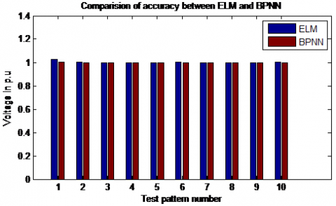
Whenever there is a disturbance the bus voltage will be deviated from reference value i.e 1 p.u. ELM based ANN or BPNN based ANN will sense the deviation and predicts the parameters of SVC such that it improves the voltage profile at the buses. With the parameter prediction by ELM algorithm the voltage is brings back to the reference value effectively which was shown in Figure 17.
Table 7. Comparison between ELM and BPNN methods with 30-bus SVC firing angle model
|
S.No |
%of change in load |
Voltage at bus-30 without SVC |
αsvc Predicted |
Elapsed Time |
Voltage at bus-30 with SVC |
|||
|
BPNN |
ELM |
BPNN |
ELM |
BPNN |
ELM |
|||
|
1 |
5 |
0.9919 |
128.2287 |
128.2072 |
0.036975 |
0.005211 |
0.9999 |
0.9992 |
|
2 |
10 |
0.9896 |
128.3032 |
128.2892 |
0.035867 |
0.000145 |
1.0000 |
0.9995 |
|
3 |
15 |
0.9872 |
128.3736 |
128.3731 |
0.033183 |
0.000083 |
0.9999 |
0.9999 |
|
4 |
20 |
0.9848 |
128.4474 |
128.4553 |
0.024665 |
0.000126 |
0.9999 |
1.0002 |
|
5 |
25 |
0.9823 |
128.5276 |
128.5388 |
0.034467 |
0.000153 |
1.0001 |
1.0004 |
|
6 |
30 |
0.9798 |
128.6051 |
128.6201 |
0.025944 |
0.00012 |
1.0001 |
1.0006 |
|
7 |
35 |
0.9774 |
128.6710 |
128.6962 |
0.036435 |
0.000076 |
0.9998 |
1.0006 |
|
8 |
40 |
0.9748 |
128.7298 |
128.7759 |
0.031359 |
0.000083 |
0.9992 |
1.0007 |
|
9 |
45 |
0.9723 |
128.7734 |
128.8500 |
0.036517 |
0.000081 |
0.9981 |
1.0006 |
|
10 |
50 |
0.9697 |
128.8073 |
128.9245 |
0.038679 |
0.000068 |
0.9966 |
1.0005 |
Figure 16. Comparison of elapsed time for pridiction of parameters of SVC Facts controller
Figure 17. Comparison of accuracy of the both algorithms
The Load on the power system continuously get varies, which leads to change in the bus voltages due to mismatch in the reactive power demand and the generation. The required parameters of the SVC FACTS controller must be tuned accurately and quickly before the load goes to the next state. In this paper optimal loactaion of the SVC FACTS controller was identified using L-index method. Two models of SVC, susceptance and firing angle models are designed and simulated. The parameters of the SVC FACTS controller are tuned with the help of BPNN and ELM algorithms. It has been observed the training time of BPNN is very high as it is an iterative procedure. At the same time is very les for ELM as it is a non-iterative procedure. Once trained with ELM algorithm the parameters of the SVC FACTS controller forcasted quicly and effectively compared with BPNN. As the BPNN suffers from network paralysis, local minima and slow convergence, these are overcome by proposed ELM algorithm.
[1] Bujal, N.R., Hasan, A.E., Sulaiman, M. (2014). Analysis of voltage stability problems in power system. 4th International conference on Engineering Technology and Technopreneuship (ICE2T), Kuala Lumpur, Malaysia, pp. 27-29. https://doi.org/10.1109/ICE2T.2014.7006262
[2] Wibowo, R.S., Yorino, N., Eghbal, M., Zoka, Y., Sasaki, Y. (2011). FACTS devices allocation with control coordination considering congestion relief and voltage stability. IEEE Transactions on Power Systems, 26(4): 2302-2310. https://doi.org/10.1109/TPWRS.2011.2106806
[3] Rahman, H., Rahman, M.F. (2012). Stability improvement of power system by using SVC with PID controller. International Journal of Emerging Technology and Advanced Engineering, 2(7): 226-233.
[4] Priyadhershni, M., Udhayashankar, C., Kumar Chinnaiyan, V. (2014). Simulation of static var compensator in IEEE 14 bus system for enhancing voltage stability and compensation. Power Electronics and Renewable Energy Systems, 326: 265-273. https://doi.org/10.1007/978-81-322-2119-7_27
[5] Pourbeik, P. (2006). Modeling and application studies for a modern static VAr system installation. IEEE Transactions on Power Delivery, 21(1): 368-376. https://doi.org/10.1109/TPWRD.2005.852382
[6] Chang, Y.C. (2012). Multi-objective optimal SVC installation for power system loading margin improvement. IEEE Transactions on Power Systems, 27(2): 984-991. https://doi.org/10.1109/TPWRS.2011.2176517
[7] Abdel-Rahman, M.H., Youssef, F.M.H., Saber, A.A. (2006). New static var compensator control strategy and coordination with under-load tap changer. IEEE Transactions on Power Delivery, 21(3): 1630-1635. https://doi.org/10.1109/TPWRD.2005.858814
[8] Harikrishna, D., Srikanth, N.V. (2012). Dynamic stability enhancement of power systems using neural-network controlled static-compensator. TELKOMNIKA, 10(1): 9-16. https://doi.org/10.11591/telkomnika.v10i1.648
[9] Abood, A.A., Tuaimah, F.M., Maktoof, A.H. (2012). Modeling of SVC controller based on adaptive PID controller using neural networks. International Journal of Computer Applications, 59(6): 9-16. https://doi.org/10.5120/9551-4007
[10] Huang, W.H., Sun, K. (2018). Optimization of SVC settings to improve post-fault voltage recovery and angular stability. Journal of Modern Power Systems and Clean Energy, 7: 491-499. https://doi.org/10.1007/s40565-018-0479-0
[11] Brito, M.E.C., Cavalcanti, M.C., Limongi, L.R., Neves, F.A.S., Azevedo, G.M.S. (2018). Adjustable VAr compensator with losses reduction in the electric system. Electrical Engineering, 100(4): 2165-2175. https://doi.org/10.1007/s00202-018-0692-x
[12] Huang, H.L., Kong, Y. (2008). The analysis on the L-index based optimal power flow considering voltage stability constraints. WSEAS Transactions on Systems, 11(7): 1300-1309. https://doi.org/10.1155/2019/2609235
[13] London, S.P., Rodriguez, L.F., Oliver, G. (2014). A simplified voltage stability index (SVSI). Electrical Power and Energy System, 63: 806-813. https://doi.org/10.1016/j.ijepes.2014.06.044
[14] Sivanandam, S.N., Sumathi, S., Deepa, S.N. (2005). Introduction to Neural Networks Using MATLAB 6.0. Tata McGraw-Hill, New Delhi.
[15] Suman, M., Venu Gopala Rao, M., Hanumaiah, A., Rajesh, K. (2016). Solution of economic load dispatch problem in power system using lambda iteration and back propagation neural network methods. International Journal on Electrical Engineering and Informatics, 8(2): 347-355. https://doi.org/10.15676/ijeei.2016.8.2.8
[16] Huang, G.B., Zhu, Q.Y., Siew, C.K. (2004). Extreme learning machine: A new learning scheme of feedforward neural networks. IEEE International Conference on Neural Networks, 2: 985-990. https://doi.org/10.1109/IJCNN.2004.1380068