OPEN ACCESS
Rotating machines are very common in industry.To understand their behaviour is therefore,very important. When considering numerical analysis of such systems, their modelling needsto consider several important effects which are normally disregarded, such as damping and stiffness coefficients associated with the hydrodynamic interactions between the shaft and the supporting bearings.
Hydrodynamic bearings play an important role in proper functioning of turbo machinery. They have a direct effect on the dynamic behaviour of this type of machine by adding stiffness to the system. In this paper harmonic analysis of the rotor is done to identify the frequency through the variation of the diameters by design of the optimization (DOE). In the DOE, two levels were used with a total of eleven diameters as parameters and four stiffness factors, which resuted in forty eight runs as per Plakett-Burman design (PBD) plan for answers. Pareto effect graphs and Main effects Plot have been studied to identify the influence of stiffness and the diameters responsible for producing major effects on frequency. We have seen that the stiffness Kyz and the diameters D4 and D10 have an effect on frequency. The results of the confirmatory tests showed that the Plackett-Burman method was very effective in optimizing of rotating machines.
stiffness, DOE, hydrodynamic bearings, dynamic behaviour, turbomachinery
DOE is a systematic approach to investigation of a system or process. A series of structured tests are designed in which planned changes are made to the input variables of a process or system. The effects of these changes on a pre-defined output are then assessed. Design of Experiments (DOE) techniques enables designers to determine simultaneously the individual and interactive effects of many factors that could affect the output results in any design. DOE also provides a full insight of inter-action between design elements; therefore, it helps turn any standard design into a robust one. Simply put, DOE helps to pin point the sensitive parts and sensitive areas in designs that cause problems in Yield. Designers are then able to fix these problems and produce robust and higher yield designs prior going into production. Turbo machines are widely employed in several industrial processes. The most common cause of vibration in turbo machines is the rotor mass unbalance. The unbalance centrifugal forces are transmitted to the machine support system and foundation. Such forces may damage the system and, in some cases, even affect others equipments in the vicinity. The use of computational procedures to analyze the dynamic behavior of turbo machines has provided significant data for the preliminary stages of the machine design. The rotating system modeling usually is based on simplified models for the support system, which commonly do not account for the hydrodynamic bearing dynamic force coefficients.
Even though the bearing coefficients play an important role on the rotor response, the lacks analyses of rotating machines that include the stiffness and damping coefficients associa Ted with the hydrodynamic journal bearings.
Regarding hydrodynamic bearings, Reynolds equation describes the hydrodynamic lubrication and defines the bearing pressure field as a function of motion (displacement and velocity) in the bearing [1-2].
Glienicke et al. [3] determined the dynamic coefficients considering four different bearing types under controlled conditions. Hashimoto et al. [4] calculated the oil film forces for short bearings using analytical formulation.
The various materials used in bearing constructions and load-carrying capacity. Values of stiffness and damping coefficients of hydrodynamic bearings are the most important from the point of view of dynamical performance [5-6]. The paper of Delgado [7] presents the identification of dynamic coefficients of a hybrid gas bearing that has a sophisticated and robust construction with a complex structure of the foils. The literature study showed that an experimental determination of stiffness and damping bearing characteristics is conducted not just for radial bearings but for thrust bearings as well.
Stiffness and damping hydrodynamic bearings coefficients can be determined using numerical formulation via finite differences and finite elements from the zero and first order Reynolds equation through perturbation analysis of the system [8-10]. Then, one of the main objectives of the researchers and designers was to be able to obtain fundamental mathematical models, adequate to the observed physical phenomena, in order to predict numerically the dynamic behavior of rotor systems and the influence of the support flexibility of rotors. In recent years, there has been an important research activity in the field of modeling and analysis of the dynamic behavior of rotating machinery in order to adjust some system parameters and to obtain the most suitable design within the speed range of interest.
Wettergren and Olsson [12] also demonstrates from a parametric study of a simplified finite element model that instabilities occur for certain combinations of parameters associated with internal damping, external damping, asymmetric tree stiffness and anisotropic / dissymmetrical bearings.
Then, the utilization of finite element models in the area of rotor dynamics was applied to develop suitable models and has yielded highly successful results [13-14]. These numerical models are now used to design machinery to operate within acceptable limits.
Taplak [15] in his paper studied a program named Dynrot was used to make dynamic analysis and the evaluation of the results. For this purpose, a gas turbine rotor with certain geometrical and mechanical properties was modeled and its dynamic analysis was made by Dynrot program.
Gurudatta [16] in his paper presented an alternative procedure called harmonic analysis to identify frequency of a system through amplitude and phase angle plots. The unbalance that exists in any rotor due to eccentricity has been used as excitation to perform such an analysis. ANSYS parametric design language has been implemented to achieve the results.
Sinou [17] investigated the response of a rotor’s non- linear dynamics which is supported by roller bearings. He studies on a system comprised of a disk with a single shaft, two flexible bearing supports and a roller bearing. He found that the reason of the exciter is imbalance. He used a numerical method named Harmonic Balance Method for this study. Chouskey [18] et al. studied the influences of internal rotor material damping and the fluid film forces (generated as a result of hydrodynamic action in journal bearings) on the modal behavior of a flexible rotor-shaft system. It is seen that correct estimation of internal friction, in general, and the journal bearing coefficients at the rotor spin-speed are essential to accurately predict the rotor dynamic behaviour.This serves as a first step to get an idea about dynamic rotor stress and, as a result, a dynamic design of rotors.
Kun Li et al. [19] a laboratory method based on equivalent dynamic load reconstruction is proposed for the identification of oil-film coefficients. When modeling the rotor, the oil-film supports are considered as its dynamic load boundary conditions. Consequently, the identification of oil-film coefficients is first con-verted to the reconstruction of equivalent dynamic loads. Through Green's function method and reg-ularization, the equivalent dynamic oil-film loads can be steadily and precisely reconstructed. Then, according to the mechanical relationships between the oil-film properties and the corresponding equivalent loads, the oil-film stiffness and damping coefficients are identified using least square scheme. A rotor structure with two journal bearings is investigated and the identification results of oil-film coefficients demonstrate the validity and accuracy of the proposed method.
Whalley and Abdul-Ameer [20], calculated the rotor resonance, critical speed and rotational frequency of a shaft that its, diameter changes by the length, by using basic harmonic response method.
Gasch [21], investigated the dynamic behavior of a Laval (Jeffcott) rotor with a transverse crack on its elastic shaft, and developed the non-linear motion equations which gave important clues on the crack diagnosis.
Das et al. [22] aimed to develop an active vibration control scheme to control the transverse vibrations on the rotor shaft arising from imbalance and they performed an analysis on the vibration control and stability of a rotor- shaft system which has electromagnetic exciters.
Villa et al. [23] studied the non-linear dynamic analysis of a flexible imbalanced rotor supported by roller bearings. They used Harmonic Balance Method for this purpose. Stability of the system was analyzed in frequency term with a method based on complexity. They showed that Harmonic Balance Method has realized the AFT strategy and harmonic solution very efficiently. Lei and Palazzolo [24] have analyzed a flexible rotor system supported by active magnetic bearings and synthesized the Campbell diagrams, case forms and eigen values to optimize the rotor-dynamic characteristics and obtained the stability at the speed range. They also investigated the rotor critical speed, case forms, frequency responses and time responses.
Ritesh Fegade and Vimal Patel et al. [25-26] in his article studied the harmonic analysis of the rotor is made to identify the frequency through variation in
diameters by optimization design (DOE) and parametric design ANSYS. In addition to other search for an alternative procedure called harmonic analysis to identify the frequency of a system through critical velocity, amplitude and phase angle curves using ANSYS.
In addition, Łukasz Breńkacz et al. [29] described experimental research. Displacement signals were shown in the bearings and excitation forces used to determine the dynamics of the carrier. The study discussed in this article deals with the rotor supported by two hydrodynamic actuators working in a nonlinear manner. On the basis of calculations, dynamic transaction results were presented for a specific speed.
Fulaj et al. [30] discusses in his research how to obtain critical speeds of the rotor carrier system. A mathematical model for the flexible column was developed with a steel rotor using a specific elementTechniques. The limited element model was used to obtain critical speeds in MATLAB.
In this paper, the harmonic analysis of the rotor is done to identify the frequency through the variation of the diameters by the design of the optimization (DOE). In the DOE, two levels were used with a total of eleven diameters and four stiffness factors as parameters, which made forty-eight tests according to the Plakett-Burman plan for answers. Pareto chart of the Standardized Effects and Normal Plot of the Standardized Effects and Main effects Plot of frequency have
been studied to identify the stiffness and the diameters that are responsible for producing major effects on frequency. It has been seen that the stiffness Kyz and the diameters D4 and D10, are responsible for producing major effects on the frequency, have a decisive impact on the dynamic behaviour of rotating machinery.
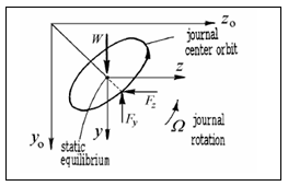
Consider that the journal moves in the bearing along an orbit around its steady-state equilibrium position Fig.1. The resultant reaction force of lubricant film has a variable magnitude and direction (it is no more vertical). Its components F y and Fzare non-linear functions of the journal center displacements y and z, and its velocity components
and :$\mathrm{F}^{y}=\mathrm{F}^{y}\left(y_{, z}, z, \dot{z}\right) \cdot \mathrm{Fz}=\mathrm{Fz}(y, z, z, \dot{z})$
For a small amplitude motion, the bearing reaction may be expressed by the first order Taylor series expansion of its components around the static equilibrium position (note the direction of the force components here, selected to avoid the “minus” sign in the following expressions):
$\mathrm{Fy}=\mathrm{Fy} 0+\mathrm{Kyy} \mathrm{y}+\mathrm{Kyz} z+\mathrm{CYY} \quad \dot{y}+\mathrm{Cyz} \dot{Z}$
$\mathrm{Fz}=\mathrm{F} \mathrm{z} 0+\mathrm{Kzy} \mathrm{y}+\mathrm{Kzz} \mathrm{z}+\mathrm{Cz} \mathrm{Y} \quad \dot{y}_{+\mathrm{Czz}} \dot{Z}$ (1)
The static reaction force components are Fyo =W and Fzo = 0.The eight coefficients of the linearized force components are computed as the gradients in the static equilibrium position
$(\mathrm{y}=\mathrm{z}=\dot{y}=\dot{z}=0) :$
$\mathrm{kyy}=\left(\frac{\partial F y}{\partial y}\right) 0, \mathrm{kyz}=\left(\frac{\partial F y}{\partial z}\right) 0, \mathrm{kzy}=\left(\frac{\partial F z}{\partial y}\right) 0, \mathrm{kzz}=\left(\frac{\partial F z}{\partial z}\right) 0$
$\mathrm{Cyy}=\left(\frac{\partial F y}{\partial \dot{y}}\right) 0, \mathrm{Cyz}=\left(\frac{\partial F y}{\partial \dot{z}}\right) 0, \mathrm{Czy}=\left(\frac{\partial F z}{\partial}\right) 0, \mathrm{Czz}=\left(\frac{\partial F z}{\partial \dot{z}}\right) 0$
They result from the solution of the lubrication equation.
The linearization of the bearing reaction forces has the advantage of decoupling the rotor and the bearings. Otherwise, the rotor equations must be integrated simultaneously with the lubrication equation.
Figure 1. Equilibrium position
In matrix form, equation (1) can be written
$\left\{\begin{array}{c}{F y} \\ {F z}\end{array}\right\}=\left\{\begin{array}{c}{W} \\ {O}\end{array}\right\}+\left\{\begin{array}{c}{\Delta F y} \\ {\Delta F Z}\end{array}\right\}$
The increments of the film force due to small movements around the position of static equilibrium are expressed in terms of stiffness and damping coefficients.
$\left\{\begin{array}{ll}{\Delta F y} \\ {\Delta F Z}\end{array}\right\}=\left[\begin{array}{ll}{k y y} & {k y z} \\ {k Z y} & {k Z Z}\end{array}\right]$$\left\{\begin{array}{l}{y} \\ {z}\end{array}\right\}+\left[\begin{array}{ll}{C y y} & {C y z} \\ {C z y} & {C z z}\end{array}\right]$$\left\{\begin{array}{l}{\dot{y}} \\ {\dot{z}}\end{array}\right\}$$=[\mathrm{K} \mathrm{b}]\left\{\begin{array}{l}{y} \\ {z}\end{array}\right\}+[\mathrm{Cb}]$$\left\{\begin{array}{c}{\dot{y}} \\ {\dot{z}}\end{array}\right\}$
The eight linearized stiffness and damping coefficients depend on the journal steady-state operating conditions, hence upon the rotational speed. The dimensionless stiffness coefficients are defined as
$[\mathrm{K} \mathrm{b}]=\left[\begin{array}{ll}{k y y} & {k y z} \\ {k z y} & {k z z}\end{array}\right]=\frac{c}{W}[\mathrm{K} \mathrm{b}]$ (3a)
While the dimensionless damping coefficients are defined as
$[\mathrm{C} \mathrm{b}]=\left[\begin{array}{cc}{\text {Cyy}} & {\mathrm{Cyz}} \\ {\mathrm{Czy}} & {\mathrm{Cyz}}\end{array}\right]=\frac{c \Omega}{w}[\mathrm{Cb}]$ (3b)
For a given set of geometrical parameters and lubricant viscosity, these eight coefficients are functions of the Sommerfeld number S or the eccentricity ratio. They are referred to as the eight dynamic bearing coefficients. Values of these coefficients are given in the book edited by Someya [23]. For flexible shafts or slightly tilted rigid journals, the journal axis may not be parallel to the bearing axis.
The pressure distribution along the journal length gives rise to reaction moments. The corresponding Taylor series expansion defines four moment stiffness coefficients and four moment damping ceofficients Generally, compared to the radial coefficients, they are smaller by a factor of (2L/ l) where l is the span adjacent to the bearing and l is the bearing length. Only for long bearings or for higher order shaft modes, the influence of moment coefficients may become significant.The stiffness matrix of journal bearings is non-symmetric. This is the cause of rotor instability above a limiting running speed called the onset speed of instability. The unstable motion of journal bearings is called oil whirl and involves large-amplitude subsynchronous motion at the rotor critical speed. Vertical rotors without side loads may experience a motion consisting of a limit cycle whose frequency tracks at approximately one-half running speed which is also called oil whirl. At speeds above twice the rotor's natural frequency, the rotor subsynchronous motion stops tracking running speed and precesses at the natural frequency, motion that is called oil whip.
The Nelson rotor is selected here for optimization. In DOE two levels are used with fifteen parameters which resulted in forty eight runs. The effects of these stiffness and diameters on the frequency are observed in the DOE. MINITAB 17 is used for this purpose.
3.1 Model
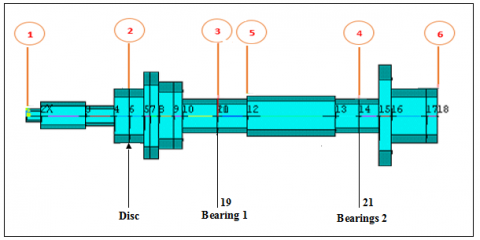
The model considered is a Nelson rotor [11]. Fig. 2, which is a 0.355 (m) long overhanging steel shaft of 14 different cross sections. The shaft carries a rotor of mass 1.401(kg) and eccentricity 0.635(cm) at 0.0889(m) from left end and is supported by firstly two bearings at a distance of 0.1651(m) and 0.287(m) from the left end respectively.
Six stations are considered during harmonic analysis as shown in Fig.1, where station numbers denote different nodes in the model (1) Left extreme of shaft, (2) Disc, (3) First bearing node, (5) Between the two bearings, (4) Second bearing node and (6) Right extreme of shaft. A density of 7806 kg/m3 and elastic modulus 2.078E11 n/m2 were used for the distributed rotor and a concentrated disk with a mass of 1.401 kg, polar inertia 0.002 kg.m2 and diametral inertia 0.00136 kg.m2 was located at station five.
Figure 2. Model of Nelson rotor with various sections, disc and bearings Numbers indicate station numbers
The following cases of bearings were analyzed:
a) Symmetric orthotropic bearings
b) Fluid film bearings.
3.2 Calculation of the Eigen values of a system
We designed a mathematical model under the name Nelson rotor in a Matlab software that contains the engineering data of the Nelson rotor element (shaft data, disk data, bearing data).
In addition to the Matrices of the stiffness and damping in the form of a set of nodes and elements to calculate the values of the existing stiffness and frequency in the presence of the speed 4800-28800 rpm. Table 1.
Table 1. Geometric data of rotor-bearing element
|
Node Location (cm) |
Bearing and Disk |
Inner Diameter (cm) |
Outer Diameter (cm) |
|
|
1 |
0.0 |
|
0.0 |
0.51 |
|
|
2 |
1.27 |
|
0.0 |
1.02 |
|
|
3 |
5.08 |
|
0.0 |
0.76 |
|
|
4 |
7.62 |
|
0.0 |
2.03 |
|
|
5 |
8.98 |
Disk |
0.0 |
2.03 |
|
|
6 |
10.16 |
|
0.0 |
3.30 |
|
|
7 |
10.67 |
|
1.52 |
3.30 |
|
|
8 |
11.43 |
|
1.78 |
2.54 |
|
|
9 |
12.70 |
|
0.0 |
2.54 |
|
|
10 |
13.46 |
|
0.0 |
1.27 |
|
|
11 |
16.51 |
Bearing |
0.0 |
1.27 |
|
|
12 |
19.05 |
|
0.0 |
1.52 |
|
|
13 |
22.86 |
|
0.0 |
1.52 |
|
|
14 |
26.67 |
|
0.0 |
1.27 |
|
|
15 |
28.70 |
|
0.0 |
1.27 |
|
|
16 |
30.48 |
|
0.0 |
3.81 |
|
|
17 |
31.50 |
|
0.0 |
2.03 |
|
|
18 |
34.54 |
|
1.52 |
2.03 |
4.1 Data of fluid film bearings
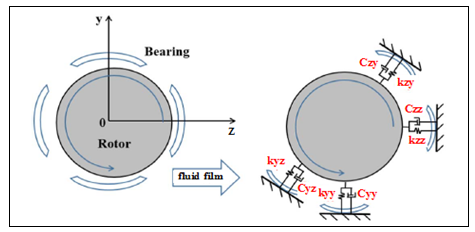
The shaft is supported by two fluid film bearings whose stiffness coefficient Fig.3 was calculated by Matlab as follows:
Factor KYY (N / m) KYZ (N / m)
Level 1 7.7539E+007 2.3381E+008
Level 2 5.8365E+008 5.8365E +008
Factor KZY (N / m) KZZ (N / m)
Level 1 -5.4601E+008 1.3399E+008
Level 2 -8.412E+007 1.4718E+008
While the damping components are Czz = Cyy = 1752 (Ns / m). The imbalance response for a disk center center eccentricity of 0.635 (cm) at station two was determined for a speed range of 4800 to 28800 rpm.
Figure 3. Schematic view of rotor on bearing supports and idealization of fluid film coefficients
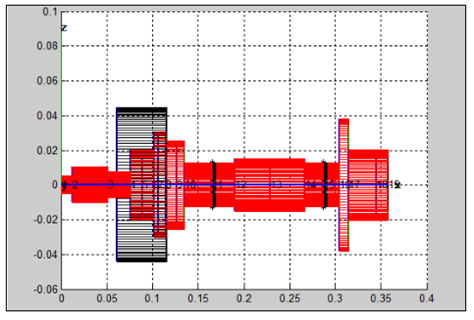
The Matlab program also provided us with a model for Nelson rotor with various sections, disc and bearings.Fig.3.
Figure 4. Nelson rotor with various sections
The Plackett – Burmann design is a very useful tool which enables to screen n variables using only n+1 experiments [28]. We use the Plackett-Burman (PBD) to improve rotor and determine the impact of stiffness on rotary machine dynamics as well as knowing the diameters responsible for producing large effects on the frequency as well the reactions which increase or decrease the main effects.Table 3 shows 48 tests required for two-level factorial design and fifteen parameters according to Plakett-Burman design (PBD) in the DOE This is after the optimization process.
The parameters used here are all the Nelson rotor diameters and four the stiffness factors. One response which is the excitation frequency is obtained for each one with the help of the matlab software. DOE is performed to discover the effect of the stiffness and the diameters on the frequency.
PBD is a design experiment that works based on the first order polynomial model:
$y=\beta_{0}+\sum \beta i X \overline{i}$ (4)
where y is the response , β0 is the model intercept, βi is the linear coefficient, and Xi is the level of the independent variable. Therefore, this model only used to screen and evaluate the important variables that significantly influence the response and does not portray interaction among variables.
The design matrix of the Plackett – Burmann at the beginning of the design for the effects of 11 diameters and 4 factors of rigidity of the experiment by DOE revealed that only 2 out of 15 factors influenced. The non-selection of the remaining thirteen factors suggests their insignificant contribution (P> 0.05) to the response studied at the confidence level selected for the study. Fig.5.
Fig .5 reveals that kyz has the greatest significant positive effect on the rightmost frequency of the response line. However, the figure reveals a significant reduction effect of kzy on the frequency of its effect is positioned to the left of the answer line.
Figure 5. Pareto chart of the standardized effect
Table 2. The Variance analysis of the regression model from the Plackett–Burmann for the estimated effects and coefficientsfor the frequency. Confirms previous results
|
Source |
DF |
Adj SS |
Adj MS |
F-Value |
P-Value |
|
Model |
15 |
523.954 |
34.930 |
6.11 |
0.000 |
|
Linear |
15 |
523.954 |
34.930 |
6.11 |
0.000 |
|
D1 |
1 |
3.586 |
3.586 |
0.63 |
0.434 |
|
D2 |
1 |
0.022 |
0.022 |
0.00 |
0.951 |
|
D3 |
1 |
4.967 |
4.967 |
0.87 |
0.358 |
|
D4 |
1 |
6.946 |
6.946 |
1.22 |
0.278 |
|
D6 |
1 |
0.002 |
0.002 |
0.00 |
0.985 |
|
D8 |
1 |
4.915 |
4.915 |
0.86 |
0.361 |
|
D10 |
1 |
0.200 |
0.200 |
0.04 |
0.853 |
|
D12 |
1 |
4.272 |
4.272 |
0.75 |
0.394 |
|
D14 |
1 |
0.227 |
0.227 |
0.04 |
0.843 |
|
D16 |
1 |
0.077 |
0.077 |
0.01 |
0.908 |
|
D17 |
1 |
6.380 |
6.380 |
1.12 |
0.299 |
|
Kyy |
1 |
5.415 |
5.415 |
0.95 |
0.338 |
|
Kyz |
1 |
353.276 |
353.276 |
61.82 |
0.000 |
|
Kzy |
1 |
133.533 |
133.533 |
23.37 |
0.000 |
|
Kzz |
1 |
0.137 |
0.137 |
0.02 |
0.878 |
|
Error |
32 |
182.862 |
5.714 |
|
|
|
Total |
47 |
706.816 |
|
|
|
Model Summary
S R-sq R-sq (adj) R-sq (pred)
2.39049 74.13% 62.00% 41.7
To improve the remaining 13 response factors so that the values are set (P <0.05), we modify the red reference line at zero by moving the matrix columns (basic design matrix) one by one manually, maintaining the corresponding frequency values for each line and maintaining the matrix balance. Up to the matrix shown in Table 3.
Table 3. Runs used in DOE
|
|
d1 |
d2 |
d3 |
d4 |
d6 |
d8 |
d10 |
d12 |
d14 |
d16 |
d17 |
KYY |
KYZ |
KZY |
KZZ |
FRQ |
|
1 |
0.0152 |
0.0154 |
0.0204 |
0.0356 |
0.071 |
0.0458 |
0.0304 |
0.0254 |
0.0304 |
0.0712 |
0.0356 |
77539000 |
233810000 |
-84120000 |
133990000 |
76.53 |
|
2 |
0.0052 |
0.0254 |
0.0102 |
0.0356 |
0.071 |
0.0558 |
0.0304 |
0.0254 |
0.0304 |
0.0712 |
0.0456 |
77539000 |
233810000 |
-84120000 |
147180000 |
76.55 |
|
3 |
0.0152 |
0.0254 |
0.0204 |
0.0456 |
0.061 |
0.0458 |
0.0204 |
0.0254 |
0.0304 |
0.0712 |
0.0356 |
135940000 |
233810000 |
-84120000 |
147180000 |
76.27 |
|
4 |
0.0152 |
0.0254 |
0.0204 |
0.0456 |
0.061 |
0.0458 |
0.0204 |
0.0254 |
0.0304 |
0.0712 |
0.0356 |
135940000 |
233810000 |
-84120000 |
147180000 |
76.27 |
|
5 |
0.0152 |
0.0254 |
0.0102 |
0.0356 |
0.061 |
0.0458 |
0.0204 |
0.0354 |
0.0204 |
0.0712 |
0.0456 |
77539000 |
233810000 |
-84120000 |
133990000 |
76.53 |
|
6 |
0.0152 |
0.0254 |
0.0102 |
0.0456 |
0.071 |
0.0458 |
0.0204 |
0.0254 |
0.0304 |
0.0812 |
0.0356 |
135940000 |
233810000 |
-84120000 |
133990000 |
76.24 |
|
7 |
0.0152 |
0.0154 |
0.0204 |
0.0356 |
0.071 |
0.0558 |
0.0204 |
0.0354 |
0.0304 |
0.0712 |
0.0456 |
135940000 |
233810000 |
-84120000 |
147180000 |
76.27 |
|
8 |
0.0152 |
0.0154 |
0.0102 |
0.0356 |
0.061 |
0.0558 |
0.0204 |
0.0354 |
0.0304 |
0.0712 |
0.0356 |
135940000 |
233810000 |
-84120000 |
133990000 |
76.24 |
|
9 |
0.0052 |
0.0254 |
0.0102 |
0.0356 |
0.071 |
0.0558 |
0.0304 |
0.0254 |
0.0304 |
0.0712 |
0.0456 |
77539000 |
233810000 |
-84120000 |
147180000 |
76.55 |
|
10 |
0.0052 |
0.0254 |
0.0102 |
0.0356 |
0.071 |
0.0558 |
0.0304 |
0.0254 |
0.0304 |
0.0712 |
0.0456 |
77539000 |
233810000 |
-84120000 |
147180000 |
76.55 |
|
11 |
0.0152 |
0.0154 |
0.0102 |
0.0356 |
0.061 |
0.0558 |
0.0204 |
0.0354 |
0.0304 |
0.0712 |
0.0356 |
135940000 |
233810000 |
-84120000 |
133990000 |
76.24 |
|
12 |
0.0152 |
0.0154 |
0.0102 |
0.0356 |
0.071 |
0.0558 |
0.0204 |
0.0254 |
0.0204 |
0.0812 |
0.0456 |
135940000 |
583650000 |
-84120000 |
133990000 |
85.35 |
|
13 |
0.0052 |
0.0154 |
0.0204 |
0.0456 |
0.071 |
0.0458 |
0.0304 |
0.0254 |
0.0304 |
0.0712 |
0.0356 |
135940000 |
583650000 |
-84120000 |
133990000 |
85.35 |
|
14 |
0.0052 |
0.0254 |
0.0204 |
0.0456 |
0.071 |
0.0558 |
0.0304 |
0.0354 |
0.0304 |
0.0712 |
0.0356 |
77539000 |
583650000 |
-546010000 |
133990000 |
85.31 |
|
15 |
0.0052 |
0.0254 |
0.0102 |
0.0356 |
0.061 |
0.0458 |
0.0304 |
0.0354 |
0.0204 |
0.0812 |
0.0456 |
135940000 |
233810000 |
-546010000 |
147180000 |
83.61 |
|
16 |
0.0152 |
0.0154 |
0.0102 |
0.0456 |
0.071 |
0.0458 |
0.0304 |
0.0254 |
0.0304 |
0.0712 |
0.0456 |
135940000 |
583650000 |
-546010000 |
147180000 |
85.01 |
|
17 |
0.0052 |
0.0154 |
0.0204 |
0.0456 |
0.061 |
0.0558 |
0.0204 |
0.0354 |
0.0304 |
0.0712 |
0.0456 |
77539000 |
233810000 |
-546010000 |
133990000 |
84.25 |
|
18 |
0.0152 |
0.0154 |
0.0204 |
0.0456 |
0.061 |
0.0458 |
0.0204 |
0.0254 |
0.0204 |
0.0812 |
0.0356 |
77539000 |
583650000 |
-84120000 |
147180000 |
86.66 |
|
19 |
0.0152 |
0.0254 |
0.0102 |
0.0456 |
0.071 |
0.0558 |
0.0304 |
0.0354 |
0.0204 |
0.0812 |
0.0356 |
77539000 |
233810000 |
-546010000 |
133990000 |
84.25 |
|
20 |
0.0152 |
0.0154 |
0.0204 |
0.0356 |
0.071 |
0.0458 |
0.0304 |
0.0254 |
0.0204 |
0.0812 |
0.0456 |
77539000 |
233810000 |
-546010000 |
147180000 |
84.12 |
|
21 |
0.0052 |
0.0154 |
0.0102 |
0.0456 |
0.061 |
0.0458 |
0.0204 |
0.0354 |
0.0204 |
0.0812 |
0.0356 |
77539000 |
583650000 |
-84120000 |
147180000 |
86.66 |
|
22 |
0.0052 |
0.0254 |
0.0204 |
0.0456 |
0.061 |
0.0558 |
0.0204 |
0.0254 |
0.0304 |
0.0812 |
0.0356 |
135940000 |
233810000 |
-546010000 |
133990000 |
83.71 |
|
23 |
0.0052 |
0.0154 |
0.0204 |
0.0356 |
0.061 |
0.0558 |
0.0304 |
0.0254 |
0.0304 |
0.0712 |
0.0456 |
135940000 |
583650000 |
-84120000 |
147180000 |
85.07 |
|
24 |
0.0152 |
0.0254 |
0.0204 |
0.0356 |
0.061 |
0.0458 |
0.0304 |
0.0354 |
0.0204 |
0.0712 |
0.0456 |
135940000 |
583650000 |
-546010000 |
147180000 |
85.01 |
|
25 |
0.0152 |
0.0254 |
0.0102 |
0.0456 |
0.061 |
0.0458 |
0.0304 |
0.0354 |
0.0304 |
0.0812 |
0.0456 |
135940000 |
583650000 |
-546010000 |
133990000 |
85.06 |
|
26 |
0.0052 |
0.0254 |
0.0204 |
0.0356 |
0.071 |
0.0558 |
0.0304 |
0.0254 |
0.0304 |
0.0812 |
0.0456 |
77539000 |
583650000 |
-546010000 |
133990000 |
85.31 |
|
27 |
0.0052 |
0.0254 |
0.0204 |
0.0456 |
0.061 |
0.0558 |
0.0204 |
0.0254 |
0.0304 |
0.0812 |
0.0356 |
135940000 |
233810000 |
-546010000 |
133990000 |
83.71 |
|
28 |
0.0052 |
0.0254 |
0.0204 |
0.0356 |
0.071 |
0.0458 |
0.0204 |
0.0254 |
0.0204 |
0.0812 |
0.0356 |
135940000 |
583650000 |
-546010000 |
147180000 |
85.01 |
|
29 |
0.0152 |
0.0254 |
0.0102 |
0.0356 |
0.061 |
0.0558 |
0.0204 |
0.0254 |
0.0204 |
0.0712 |
0.0456 |
135940000 |
583650000 |
-546010000 |
133990000 |
85.06 |
|
30 |
0.0152 |
0.0154 |
0.0102 |
0.0356 |
0.071 |
0.0558 |
0.0204 |
0.0254 |
0.0204 |
0.0812 |
0.0456 |
135940000 |
583650000 |
-84120000 |
133990000 |
85.35 |
|
31 |
0.0152 |
0.0154 |
0.0204 |
0.0356 |
0.061 |
0.0558 |
0.0304 |
0.0254 |
0.0204 |
0.0712 |
0.0456 |
77539000 |
583650000 |
-84120000 |
147180000 |
86.66 |
|
32 |
0.0052 |
0.0154 |
0.0204 |
0.0456 |
0.071 |
0.0458 |
0.0304 |
0.0254 |
0.0304 |
0.0712 |
0.0356 |
135940000 |
583650000 |
-84120000 |
133990000 |
85.35 |
|
33 |
0.0152 |
0.0154 |
0.0204 |
0.0356 |
0.071 |
0.0458 |
0.0304 |
0.0254 |
0.0204 |
0.0812 |
0.0456 |
77539000 |
233810000 |
-546010000 |
147180000 |
84.12 |
|
34 |
0.0152 |
0.0254 |
0.0102 |
0.0456 |
0.071 |
0.0558 |
0.0304 |
0.0354 |
0.0204 |
0.0812 |
0.0356 |
77539000 |
233810000 |
-546010000 |
133990000 |
84.25 |
|
35 |
0.0152 |
0.0254 |
0.0102 |
0.0356 |
0.061 |
0.0558 |
0.0304 |
0.0354 |
0.0204 |
0.0812 |
0.0356 |
77539000 |
583650000 |
-546010000 |
147180000 |
85.25 |
|
36 |
0.0052 |
0.0154 |
0.0204 |
0.0456 |
0.061 |
0.0558 |
0.0204 |
0.0354 |
0.0304 |
0.0712 |
0.0456 |
77539000 |
233810000 |
-546010000 |
133990000 |
84.25 |
|
37 |
0.0052 |
0.0254 |
0.0204 |
0.0356 |
0.071 |
0.0558 |
0.0304 |
0.0354 |
0.0204 |
0.0712 |
0.0456 |
135940000 |
233810000 |
-546010000 |
147180000 |
83.61 |
|
38 |
0.0152 |
0.0254 |
0.0204 |
0.0456 |
0.061 |
0.0558 |
0.0304 |
0.0354 |
0.0304 |
0.0812 |
0.0356 |
77539000 |
583650000 |
-546010000 |
147180000 |
85.25 |
|
39 |
0.0152 |
0.0254 |
0.0102 |
0.0456 |
0.071 |
0.0458 |
0.0304 |
0.0354 |
0.0204 |
0.0712 |
0.0456 |
77539000 |
583650000 |
-546010000 |
147180000 |
85.25 |
|
40 |
0.0152 |
0.0154 |
0.0204 |
0.0456 |
0.071 |
0.0558 |
0.0204 |
0.0354 |
0.0304 |
0.0812 |
0.0356 |
77539000 |
583650000 |
-546010000 |
133990000 |
85.31 |
|
41 |
0.0052 |
0.0154 |
0.0102 |
0.0456 |
0.061 |
0.0458 |
0.0204 |
0.0354 |
0.0204 |
0.0812 |
0.0356 |
77539000 |
583650000 |
-84120000 |
147180000 |
86.66 |
|
42 |
0.0052 |
0.0254 |
0.0102 |
0.0356 |
0.061 |
0.0458 |
0.0304 |
0.0354 |
0.0204 |
0.0812 |
0.0456 |
135940000 |
233810000 |
-546010000 |
147180000 |
83.61 |
|
43 |
0.0052 |
0.0154 |
0.0102 |
0.0456 |
0.061 |
0.0458 |
0.0204 |
0.0354 |
0.0204 |
0.0812 |
0.0356 |
77539000 |
583650000 |
-84120000 |
147180000 |
86.66 |
|
44 |
0.0052 |
0.0254 |
0.0204 |
0.0456 |
0.061 |
0.0558 |
0.0204 |
0.0254 |
0.0204 |
0.0712 |
0.0356 |
77539000 |
583650000 |
-84120000 |
133990000 |
86.97 |
|
45 |
0.0052 |
0.0154 |
0.0102 |
0.0456 |
0.061 |
0.0458 |
0.0204 |
0.0354 |
0.0204 |
0.0812 |
0.0356 |
77539000 |
583650000 |
-84120000 |
147180000 |
86.66 |
|
46 |
0.0052 |
0.0154 |
0.0204 |
0.0456 |
0.071 |
0.0458 |
0.0304 |
0.0254 |
0.0304 |
0.0712 |
0.0356 |
135940000 |
583650000 |
-84120000 |
133990000 |
85.35 |
|
47 |
0.0052 |
0.0154 |
0.0102 |
0.0356 |
0.071 |
0.0458 |
0.0204 |
0.0354 |
0.0204 |
0.0812 |
0.0456 |
135940000 |
233810000 |
-546010000 |
133990000 |
83.71 |
|
48 |
0.0052 |
0.0154 |
0.0102 |
0.0356 |
0.071 |
0.0458 |
0.0204 |
0.0354 |
0.0204 |
0.0812 |
0.0456 |
135940000 |
233810000 |
-546010000 |
133990000 |
83.71 |
5.1 The result of Plackett-Burman design
5.1.1 Analysis of variance
The main output from an analysis of variance study arranged in a tables.4.5.6 Lists the sources of variation, their degrees of freedom, the total sum of squares, and the mean squares.
The analysis of variance table also includes the F-statistics and p-values. Use these to determine whether the predictors or factors are significantly related to the response.
Table 4. Estimated effects and coefficients for frequency (coded units)
|
Source |
DF |
Adj SS |
Adj MS |
F-Value |
P-Value |
|
Model |
15 |
673.046 |
44.870 |
53930.87 |
0.000 |
|
Linear |
15 |
673.046 |
44.870 |
53930.87 |
0.000 |
|
D1 |
1 |
35.420 |
35.240 |
42355.93 |
0.000 |
|
D2 |
1 |
40.965 |
40.956 |
49227.31 |
0.000 |
|
D3 |
1 |
6.421 |
6.421 |
7717.45 |
0.000 |
|
D4 |
1 |
43.586 |
43.586 |
52387.78 |
0.000 |
|
D6 |
1 |
9.722 |
9.722 |
11684.95 |
0.000 |
|
D8 |
1 |
15.850 |
15.850 |
19050.96 |
0.000 |
|
D10 |
1 |
22.015 |
22.015 |
26461.00 |
0.000 |
|
D12 |
1 |
3.298 |
3.298 |
3963.52 |
0.000 |
|
D14 |
1 |
88.000 |
88.000 |
106562.24 |
0.000 |
|
D16 |
1 |
10.240 |
10.240 |
12307.32 |
0.000 |
|
D17 |
1 |
4.065 |
4.065 |
4885.40 |
0.000 |
|
Kyy |
1 |
3.654 |
3.654 |
4392.20 |
0.000 |
|
Kyz |
1 |
107.786 |
107.786 |
129552.46 |
0.000 |
|
Kzy |
1 |
22.016 |
22.016 |
4885.40 |
0.000 |
|
Kzz |
1 |
4.155 |
4.155 |
4392.20 |
0.000 |
|
Error |
32 |
0.027 |
0.001 |
|
|
|
Lack-of-Fit |
16 |
0.027 |
0.002 |
|
|
|
Pure Error |
16 |
0.000 |
0.000 |
|
|
|
Total |
47 |
673.072 |
|
|
|
Model Summary : S : 0.0288442 ; R-sq : 100.00% ; R-sq (adj): 99.99% ; PRESS : 0.0666097 ; R-sq (pred) : 99.99%.
The main output from an analysis of variance study arranged in a table. DF, degrees of freedom ; SS, sum of squares ; MS, mean sum of squares.Lists the sources of variation, their degrees of freedom, the total sum of squares, and the mean squares.
Table 5. Analysis of Variance for frequency (coded units)
|
Source |
DF |
Adj SS |
Adj MS |
F-Value |
P-Value |
|
Model |
15 |
673.046 |
44.870 |
53930.87 |
0.000 |
|
Obs |
FRQ |
Fit |
Resid |
Std Resid |
|
23 |
85.0700 |
85.1203 |
-0.0503 |
- 2.11 R |
|
39 |
85.2500 |
85.1993 |
0.0507 |
2.22 R |
|
44 |
86.9700 |
86.9213 |
0.0487 |
2.16 R |
The complete model, which includes both main effects and two-way interaction. We used the (P) values in the effects and coefficients estimates Table 5. To determine the significant effects. Using α = 0.05, the main effects for diameters D1 to kzz and their interactions are statistically significant; that is, their p-values are less than 0.05.
R denotes an observation with a large standardized residual.
Next, we do evaluate the normal probability curve and the Pareto curve of the standardized effects to see which effects influence the response, the excitation frequency. Significant terms are identified by a square symbol. Fig.6.
Stiffness kyz and Diameters D4 and D10 and their interactions are all significant (α = 0.05).
Figure 6. Normal plot of the standardized effect
Minitab displays the absolute value of the effects on the Pareto chart as shown in Fig.7. Any effects that extend beyond the reference line are significant at the default level of 0.05. Stiffness kyz and Diameters D4 and D10 their interactions are all significant (α = 0.05).
Figure 7. Pareto chart of the standardized effects
The regression equation in Uncoded Units Eq (5). The equation reveals that stiffness kyz has the coefficient that is preceded by a positive sign, confirming once again its strong enhancement effect on frequency.
$\mathrm{FRQ}=71.343-173.726 \mathrm{d} 1-232.72 \mathrm{d} 2+96.54 \mathrm{d} 3$
$+287.83 \mathrm{d} 4-108.81 \mathrm{d} 6+143.05 \mathrm{d} 8$
$+184.48 \mathrm{d} 10-70.92 \mathrm{d} 12-389.51 \mathrm{d} 14+127.84 \mathrm{d} 16$
$+86.30 \mathrm{d} 17+0.000000 \mathrm{KYY}$
$+0.00000 \mathrm{KYZ}-0.00000 \mathrm{KZY}-0.00000 \mathrm{KZZ}$ (5)
Then, the main effect plots are drawn in MINITAB 17 as shown in Fig.8. The effect of the stiffness and the different diameters on the excitation frequency shows, the stiffness kyz and the diameters D4 and D10 both increase the excitation frequency. The plot also states that:
• The kyz stiffness has more effect on the frequency compared to D4 and D10.
• Other diameters and other stiffness do not greatly affect the excitation frequency.
An interaction plot Fig.9 shows the impact that changing the settings of one factor has on another factor. Because an interaction can amplify or diminish the main effects, evaluating interactions is extremely important.
The parallel lines in an interaction graph indicate no interaction. The greater the difference in slope between the lines, the higher the degree of interaction. However, the interaction plot doesn't tell you if the interaction is statistically significant.
Figure 8. Main effects plot for frequency
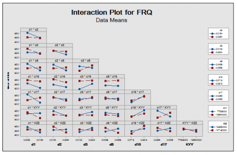
Figure 9. Interaction plot for frequency
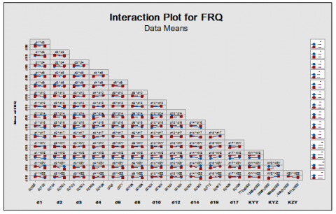
Figure 10. Interaction plot for frequency plot to visualize possible interactions
When the effect of a one factor depends on the level of the other factor. You can use an interaction plot to visualize possible interactions. Fig.10.
The plot shows that the interaction of D2 and D8 has a greater slope difference between the lines. We can thus conclude that when the values of D2 vary from 0.0154 to 0.0254, the frequency decreases, whereas when the values of D8 increase from 0.0458 to 0.0558, the frequency increases. Similarly, the interactions D1 and D8 show a similar effect: as the values of D1 increase, the frequency decreases and as the value of D8 increases, the frequency increases.
The interaction of D3 and kzz shows the similar effect that is as D3 values increases frequency increases and as kzz value increases frequency decreases.
Similarly, D1 and D17 show the same type of interaction as the D1 values increases the frequency decreases and as the D17 value increases the frequency increases.
We follow the same approach in analysis the results of interactions (d1, kzz), (d2, kzz), (d3, d8), (d3, kzz), (d8, kzz),
(d16, kzz), (d17, kyy), (d17, kzz) which can increase or decrease the frequency.
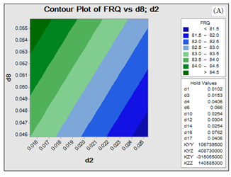
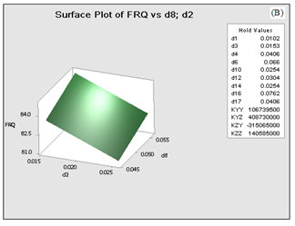
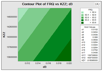
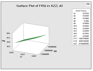
5.2 Contour and surface plots for frequency
Frequency response curves were made with the vertical axis representing the value of the frequency (Y) and the horizontal axis representing the most binary interaction (x1, x2) = (d2, d8) and (x1, x2) = (d3, kzz).The contour (A) and the surface (B) in Fig. 11 and Fig.12 show that the frequency is greater than 84.5 when d8 values The same analysis of the interaction (d3, kzz) the frequency values are less than 82.4 when the kzz stiffness values increase, and are greater than 83.6 when d3 values increase this confirms the results obtained in Fig 10.
We took a sample (d2, d8) and (d3, kzz). The same method is used to confirm the results of interactions (d1, d8) and interactions (d1, d17), (d1, kzz), (d2, kzz), (d3, d8), (d3, kzz), (d8, kzz), (d16, kzz), (d17, kyy), (d17, kzz).
Figure 11. Contour (A) and surface (B) plots of two-way interactions (d2, d8) corresponding to the frequency
Figure 12. Contour (A) and surface (B) plots of two-way interactions (d3, kzz) corresponding to the frequency
In this research, the Plackett-Burman method in DOE was used to optimize the rotor and determine the influence of stiffness on the dynamics of rotating machines in addition to knowing the diameters responsible for producing large effects on the frequency as well as the reactions which increase or decrease the main effects. Where we found:
kyz It has the greatest significant positive effect on the frequency because it appears on the right of the response line Compared to kzy, kzz which has a negative impact on the frequency and is to the left of the line of response, as confirmed by the graphs and the results of the analyzes.
The Pareto effect and design diagrams have shown that diameters D4, D10 are responsible for the production of high frequency effects.
The interaction between the factor and the other can increase or decrease the main effects as confirmed by interaction graphs and surface graphs.
These results show that the inclusion of the stiffness coefficients on the dynamic analysis of rotating machines supported on hydrodynamic bearings plays an important role on the determination of the unbalance response of rotors.
Kyy, Kyz, Kzy, Kzz = stiffness coefficients.
Cyy, Cyz, Czy, Czz = damping coefficients.
Fy , Fz are non-linear functions of the journal center.
$\dot{y}, \dot{Z}$ velocity components.
Fy0 , Fz 0 reaction force components.
[K b] dimensionless stiffness coefficients.
[C b] dimensionless damping coefficients.
Y The response .
β0 The model intercept.
βi The linear coefficient.
Xi The level of the independent variable.
Source - indicates the source of variation, either from the factor, the interaction, or the error. The total is a sum of all the sources.
DF - degrees of freedom from each source. If a factor has three levels, the degrees of freedom is 2 (n-1). If you have a total of 30 observations, the degrees of freedom total is 29 (n - 1).
SS - sum of squares between groups (factor) and the sum of squares within groups (error).
MS - mean squares are found by dividing the sum of squares by the degrees of freedom.
F - calculate by dividing the factor MS by the error MS; you can compare this ratio against a critical F found in a table or you can use the p-value to determine whether a factor is significant.
P - use to determine whether a factor is significant ; typically compare against an alpha value of 0.05. If the p-value is lower than 0.05, then the factor is significant.
[1] Childs D. (1993). Turbomachinery Rotordynamics. John Wiley & Sons, Inc, New York.
[2] Vance JM. (1988). Rotordynamics of turbomachinery. John Wiley & Sons, Inc, New York.
[3] Glienicke JDC, Han Leonhard M. (1980). Practical determination and use of bearing dynamic coefficients. Tribology International, ASME, 297–309.
[4] Hashimoto H, Wada S, Ito JI. (1987). An application of short bearing theory to dynamic characteristic problems of turbulent journal bearings. Journal of Tribology, Transactions ASME 109: 307–314. https://doi.org/10.1115/1.3261357
[5] Kiciński J. (2005). Dynamics of rotors and slide bearings (in Polish). Gdańsk: IMP PAN, Maszyny Przepływowe 2005. https://doi.org/10.1115/1.3261324
[6] Kiciński J, Żywica G. (2014). Steam Microturbines in Distributed Cogeneration. Springer monograph 2014. https://doi.org/10.1007/978-3-319-12018-8
[7] Delgado A. (2015). Experimental identification of dynamic force coefficients for a 110 mm compliantly damped hybrid gas bearing. Journal of Engineering for Gas Turbines and Power 137(7): 72502–8. https://doi.org/10.1115/1.4029203
[8] Lund W. (1987). Review of the concept of dynamic coefficients for fluid film journal bearings. ASME Journal of Tribology 109(1): 37–41. https://doi.org/10.1115/1.3261324
[9] Faria MTC. (2001). Some performance characteristics of high speed gas lubricated Herringbone groove journal bearings. JSME International Journal Series C, 44(3): 775–781. https://doi.org/10.1299/jsmec.44.775
[10] Faria MTC. (2002). A Finite element procedure for gas lubricated journal bearings. V SIMMEC, Proceedings of the Computational Mechanics Symposium (Simpósio Mineiro de Mecânica Computacional), Juiz de Fora/MG, Brazil.
[11] Nelson HD. (1976). The dynamics of rotor bearing system using finite elements. ASME Journal of Engineering for Industry 98(2): 593-60. https://doi.org/10.1115/1.3438942
[12] Wettergren HL, Olsson KO. (1996). Dynamic instability of a rotating asymmetric shaft with internal viscous damping supported in anisotropic bearings. Journal of Sound and Vibration, Academic Press Limited 195(1): 75–84. https://doi.org/10.1006/jsvi.1996.0404
[13] Lees AW, Friswell MI. (1997). The evaluation of rotor imbalance in flexibly mounted machines. Journal of Sound and Vibration 208(5): 671–683. https://doi.org/10.1006/jsvi.1997.1260
[14] V´azquez JA, Barrett LE, Flack RD. (2001). A flexible rotor on flexible bearing supports: Stability and unbalance response. Journal of Vibration and Acoustics 123(2): 137–144. https://doi.org/10.1115/1.1355244
[15] Taplak H, Parlak M. (2012). Evaluation of gas turbine rotor dynamic analysis using the finite element method. Measurement 45: 1089–1097. https://doi.org/10.1016/j.measurement.2012.01.032
[16] Gurudatt B, Seetharamu S, Sampathkumaran PS, Krishna V. (2010). Implementation, of ansys parametric design language for the determination of critical speeds of a fluid film bearing supported multi sectioned rotor with residual unbalance through modal and out of balance response analysis. Proceedings of the World Congress on Engineering Vol II.
[17] Sinou R, Baranger TN, Chatelet E, Jacquet G. (2008). Dynamic analysis of a rotating composite shaft. Composites Science and Technology 68(2): 337–345. https://doi.org/10.1016/j.compscitech.2007.06.019
[18] Chouksey M, Dutt JK, Modak SV. (2012). Modal analysis of rotor-shaft system under the influence of rotor-shaft material damping and fluid film forces. Mechanism and Machine Theory 48: 81–93. https://doi.org/10.1016/j.mechmachtheory.2011.09.001
[19] Li K, Liu J, Han X, Jiang C, Qin HJ. (2016). Identification of oil-film coefficients for a rotor-journal bearing system based on equivalent load reconstruction. Tribology International 104(2016): 285–293. https://doi.org/10.1016/j.triboint.2016.09.012
[20] Whalley R, Abdul-Ameer A. (2009). Contoured shaft and rotor dynamics. Mechanism and Machine Theory 44(4): 772–783. https://doi.org/10.1016/j.mechmachtheory.2008.04.010
[21] Gasch R. (2008). Dynamic behaviour of the Laval rotor with a transversecrack. Mechanical Systems and Signal Processing 22(4): 790–804. https://doi.org/10.1016/j.ymssp.2007.11.023
[22] Das AS, Nighil MC, Dutt JK, Irretier H. (2008). Vibration control and stability analysis of rotor-shaft system with electromagnetic exciters. Mechanism and Machine Theory 43(10): 1295–1316. https://doi.org/10.1016/j.mechmachtheory.2007.10.007
[23] Villa C, Sinou JJ, Thouverez F. (2008). Stability and vibration analysis of a complex flexible rotor bearing system. Communications in Nonlinear Science and Numerical Simulation 13(4): 804–821. https://doi.org/10.1016/j.cnsns.2006.06.012
[24] Lei SA. (2008). Control of flexible rotor systems with active magnetic bearings. Journal of Sound and Vibration 314(1–2): 19–38. https://doi.org/10.1016/j.jsv.2007.12.028
[25] Fegade R, Patel V. (2013). Unbalanced response and design optimization of rotor by ansys and design of experiments. International Journal of Scientific & Engineering Research 4(7), ISSN 2229-5518.
[26] Fegade R, Patel V, Nehete RS, Bhandarkar BM. (2014). Unbalanced response of rotor using ansys parametric design for different bearings. International Journal of Engineering Sciences & Emerging Technologies 7(1): 506-515.
[27] Someya T. (ed), Journal-Bearing Databook, Springer, Berlin, 1988.
[28] Myers RH, Montgomery DC. (1995). Response surface methodology. Process and Product Optimization Using Designed Experiments. John Wiley&Sons, Inc., NY, USA.
[29] Breńkacz Ł, Eng. Grzegorz Ż, Marta Drosińska K. (2017). the experimental identification of the dynamic coefficients of two hydrodynamic journal bearings operating at constant rotational speed and under nonlinear conditions. Polish Maritime Research 4(96): 108-115. https://doi.org/10.1515/pomr-2017-0142
[30] Fulaj D, Jegadeesan K, Shravankumar C. (2018). Analysis of a rotor supported in bearing with gyroscopic effects. IOP Conf. Series: Materials Science and Engineering 402(2018): 012059. https://doi.org/10.1088/1757-899X/402/1/012059