OPEN ACCESS
The transient flow formation due to sudden application of constant circumferential pressure gradient in an annulus partially filled with porous material has been considered. An exact solution of the governing equations has been obtained in Laplace domain using Laplace transform technique. Using suitable transformations, the equations are converted into standard Bessel equations whose solutions are available in the literature. The solutions to the Bessel equations are then inverted to the time domain using Riemann-sum approximation approach. The implicit finite difference scheme has also been employed in solving the governing equations in other to establish the accuracy of the Riemann-sum approximation approach for both transient and steady state solutions. The obtained solutions are then analysed for various dimensionless parameters entering the unified problem. There is a clear indication that large value of Da enhances the permeability of the porous region. Also, thin clear fluid region boosts $\tau_{1}$ but has no significant influence on $\tau_{\lambda}$ While thin porous region enhances skin friction at both surfaces.
annulus, circumferential pressure gradient, porous material, riemann-sum approximation, azimuthal pressure gradient
Transport processes in horizontal coaxial impermeable and non-rotating cylinders filled with composite fluid containing clear fluid and fluid-saturated porous material has been of interest in many research. This can be attributed to its immense applications in engineering such as thermal insulation, crude oil extraction processes and in biomedical systems where circumferential flow appear in most of the apparatuses conveying fluids. A theoretical investigation of laminar steady flow in a cylindrical annulus, due to a constant circumferential pressure gradient, was first studied by Dean [1], using the thin gap approximation. Analytical study on oscillatory flow in various geometries has been investigated by a number of researchers, due to an imposed oscillatory pressure gradient such as in a parallel plates by Dryden et al. [2], in circular geometry by Richardson and Tyler [3], Gupta and Gupta [4], Samal and Biswal [5]. In a rectangular geometry by Drake [6], Fan and Chao [7]. In an elliptical geometry by Khamrui [8], Haslam and Zamir [9]. Most importantly in an annular geometry by Tsangaris [10]. Recently, Tsagaris and Vlachakis [11] obtained an analytical solutions of the equations of motion of a Newtonian fluid for the fully developed laminar flow between two concentric cylinders when an oscillating circumferential pressure gradient of cyclic frequency and amplitude is imposed (finite gap oscillating Dean flow) and obtained that an increase of the reduced frequency causes a reduction of the velocity amplitude. Tsangaris et al. [12] extended the problem to the case when the walls of the cylinders are porous. The influence of the stress jump condition at the porous/clear fluid interface for steady fully developed fluid flow in a composite channel partially filled with porous material was studied by Kuznetsov [13]. Later on, Avramenko and Kuznetsov [14] studied start-up flow in a channel or pipe occupied by a fluid-saturated porous medium. They investigated the response of incompressible fluid in a parallel-plate channel or circular pipe occupied by a fluid-saturated porous medium to a suddenly applied time-dependent pressure drop.
Using semi-analytical approach, Jha and Odengle [15] examined unsteady Couette flow in a composite channel partially filled with porous material. They employed the implicit finite difference scheme in solving the governing equations and further presented a table to establish the accuracy of the Riemann-sum approach. A year later, they performed a similar analysis in a concentric cylinder, where the flow is induced by pressure gradient applied in the axial direction (See Jha and Odengle [16])). They obtained that the adjustable coefficient in the stress jump condition (β) plays an important role in flow formation.
Paul and Singh [17] discussed laminar fully developed free convection flow between two coaxial vertical cylinders partially filled with a porous matrix when the cylinders are kept at different temperatures they observed that velocity is influenced by the shear stress jump at the interface while the stability of viscous flow in a curved channel driven by a constant azimuthal pressure gradient was examined by Gibson and Cook [18]. They considered two cases of disturbances (axisymmetric and asymmetric) for finite-gap width and the narrow-gap limit and obtained that as the gap width decreases the critical mode of instability changes so that there is a transition from axisymmetric instabilities. Most recently, the effect of a radial temperature gradient on the stability of viscous flow between two porous concentric cylinders driven by a constant azimuthal pressure gradient was investigated by Deka et al. [19] using the usual Runge-Kutta scheme combined with a shooting method. It is found that for a given value of N the radially outward flow has a stabilizing effect and the stabilization is more as the gap between the cylinders increases.
Andersson and Tiseth [20] considered start-up flow in a pipe following the sudden imposition of a constant flow rate. They detected that the start-up time required to reach steady state was significantly shorter than if the start-up flow ensued from a sudden constant pressure gradient and also obtained that the solution obtained those not display the “Annular Jet Effect” seen experimentally in the work of Kataoka et al. [21].
The analytical solution of time dependent, laminar, viscous flow of an incompressible, Newtonian fluid driven by a harmonically oscillating pressure gradient in straight elliptic coaxial cylinders was investigated by Gupta et al. [22] and also presented a stepwise procedure for their evaluation for large complex arguments typically associated with viscous flows. Other related articles include the work of (Mishra and Roy [23], Chikh et al. [24], Chikh et al. [25], Chandrasekhar [26], Rajgopal et al. [27], Biswal and Mishra [28], Qi and Jin [29], Nazar et al. [30]).
The unique feature of this work is to present the semi-analytical solution of the circumferential pressure driven flow and the influence of shear stress jump condition at the interface between a clear fluid and fluid-saturated porous material. We also set to investigate the impact of variation of the interfacial radial distance on the flow formation. In this research, the solutions of the governing equations are obtained by using the Laplace transform technique, while the Riemann-sum approximation approach is used to invert the Laplace-domain solution to time-domain.
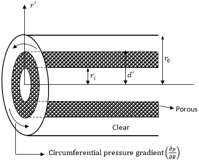
Consider the motion of transient, fully developed and incompressible circumferential flow due to Azimuthal pressure gradient between two co-axial-horizontal cylinders containing fluid and porous layer separated by a permeable thin interface with fluid occupying the interval $r_{i} \leq r^{\prime} \leq d^{\prime}$ while the interval $d^{\prime} \leq r^{\prime} \leq r_{0}$ is occupied by a fluid-saturated porous material of uniform permeability.
and are the radii of the inner and the outer cylinder respectively as shown in Fig. 1. The circumferential velocity component of the fluid is proved to be a function of the radial coordinate and time only. Following the work of Tsangaris and Vlachakis [11], the fundamental model governing the present physical situation in dimensional form can be written as follows.Figure 1. Flow configuration and coordinate system
$\frac{\partial u_{p}^{\prime}}{\partial t^{\prime}}=v_{e f f}\left[\frac{\partial^{2} u_{p}^{\prime}}{\partial r^{\prime 2}}+\frac{1}{r^{\prime}} \frac{\partial u_{p}^{\prime}}{\partial r^{\prime}}-\frac{u_{p}^{\prime}}{r^{\prime 2}}\right]-\frac{v}{k^{\prime}} u_{p}^{\prime}-\frac{1}{\rho} \frac{\partial p}{\partial \theta} \frac{1}{r^{\prime}}$ for $r_{i} \leq r^{\prime} \leq d^{\prime}$ (1)
$\frac{\partial u_{f}^{\prime}}{\partial t^{\prime}}=v\left[\frac{\partial^{2} u_{f}^{\prime}}{\partial r^{\prime 2}}+\frac{1}{r^{\prime}} \frac{\partial u_{f}^{\prime}}{\partial r^{\prime}}-\frac{u_{f}^{\prime}}{r^{\prime 2}}\right]-\frac{1}{\rho} \frac{\partial p}{\partial \theta} \frac{1}{r^{\prime}} \quad$ for $\quad d^{\prime} \leq r^{\prime} \leq r_{0}$ (2)
The initial and the no-slip condition at the surfaces for the problem under consideration are
$t^{\prime} \leq 0 : u_{p}^{\prime}=u_{f}^{\prime}=0$ for $r_{i} \leq r^{\prime} \leq r_{0}$
$t^{\prime}>0 :\left[\begin{array}{l}{u_{p}^{\prime}=0 \text { at } r^{\prime}=r_{i}} \\ {u_{f}^{\prime}=0 \text { at } r^{\prime}=r_{0}}\end{array}\right]$ (3)
With the dimensional matching condition at the interface given as
$t^{\prime}>0 :\left[\begin{array}{l}{u_{p}^{\prime}=u_{f}^{\prime}=u_{i}^{\prime}} \\ {\text {veff}\left[\frac{\partial u_{p}^{\prime}}{\partial r^{\prime}}-\frac{u_{p}^{\prime}}{r^{\prime}}\right]-v\left[\frac{\partial u_{f}^{\prime}}{\partial r^{\prime}}-\frac{u_{f}^{\prime}}{r^{\prime}}\right]=\frac{\beta v}{\sqrt{k^{\prime}}} u_{p}^{\prime}}\end{array}\right]$ at $r^{\prime}=d^{\prime}$
Introducing the following dimensionless quantities in Eqs. (1) – (3)
$R=\frac{r^{\prime}}{r_{i}} ; t=\frac{v t^{\prime}}{r_{i}^{2}} ; \gamma=\frac{v_{e f f}}{v} ; D a=\frac{r_{i}^{2}}{k^{\prime}} ; U_{p}=U_{f}=\frac{\left(u_{p}^{\prime} ; u_{f}^{\prime}\right)}{U_{0}}$
$U_{0}=-r_{i} \frac{\partial p}{\partial \theta} \frac{1}{\rho v} ; d=\frac{d^{\prime}}{r_{i}} ; \lambda=\frac{r_{0}}{r_{i}} ; U_{i}=\frac{u_{i}^{\prime}}{U_{0}}$ (4)
Equations (1) and (2) can be written in dimensionless form as
$\frac{\partial U_{p}}{\partial t}=\gamma\left[\frac{\partial^{2} U_{p}}{\partial R^{2}}+\frac{1}{R} \frac{\partial U_{p}}{\partial R}-\frac{U_{p}}{R^{2}}\right]-\frac{U_{p}}{D a}+\frac{1}{R}$ for $1 \leq R \leq d$ (5)
$\frac{\partial U_{f}}{\partial t}=\left[\frac{\partial^{2} U_{f}}{\partial R^{2}}+\frac{1}{R} \frac{\partial U_{f}}{\partial R}-\frac{U_{f}}{R^{2}}\right]+\frac{1}{R} \quad$ for $\quad d \leq R \leq \lambda$ (6)
Subject to the following non-dimensional initial and boundary condition
$t \leq 0 : U_{p}=U_{f}=0$ for $1 \leq R \leq \lambda$
$t>0 :\left[\begin{array}{l}{U_{p}=0 \text { at } R=1} \\ {U_{f}=0 \text { at } R=\lambda}\end{array}\right]$ (7)
With the non-dimensional matching condition at the interface given as
$t>0 :\left[\begin{array}{l}{U_{p}=U_{f}=U_{i}} \\ {\gamma\left[\frac{\partial U_{p}}{\partial R}-\frac{U_{p}}{R}\right]-\left[\frac{\partial U_{f}}{\partial R}-\frac{U_{f}}{R}\right]=\frac{\beta}{\sqrt{D a}} U_{p}}\end{array}\right]$ at $R=d$
The expression of equation $(5)$ to $(7)$ in Laplace domain using the Laplace transform technique $\overline{U}_{p}(\mathrm{R}, \eta)=\int_{0}^{\infty} U_{p}(R, t) e^{-\eta t} d t$ and $\overline{U}_{f}(R, \eta)=\int_{0}^{\infty} U_{f}(R, t) e^{-\eta t} d t$ (Where $\eta>0$ is the Laplace parameter) subject to initial condition yield:
$\frac{d^{2} \overline{U}_{p}}{d R^{2}}+\frac{1}{R} \frac{d \overline{U}_{p}}{d R}-\frac{\overline{U}_{p}}{R^{2}}-\frac{1}{\gamma}\left[\frac{1}{D a}+\gamma\right] \overline{U}_{p}=-\frac{1}{\gamma \eta R}$ (8)
$\frac{d^{2} \overline{U}_{f}}{d R^{2}}+\frac{1}{R} \frac{d \overline{U}_{f}}{d R}-\frac{\overline{U}_{f}}{R^{2}}-\eta \overline{U}_{f}=-\frac{1}{\eta R}$ (9)
Subject to the following non-dimensional boundary condition
$t>0 :\left[\begin{array}{l}{\overline{U}_{p}=0 \text { at } R=1} \\ {\overline{U}_{f}=0 \text { at } R=\lambda}\end{array}\right]$ (10)
With the non-dimensional matching condition at the interface given as
$t>0 :\left[\begin{array}{c}{\overline{U}_{p}=\overline{U}_{f}=U_{i}} \\ {\gamma\left[\frac{d \overline{U}_{p}}{d R}-\frac{\overline{u}_{p}}{R}\right]-\left[\frac{d \overline{U}_{f}}{d R}-\frac{\overline{U}_{f}}{R}\right]=\frac{\beta}{\sqrt{D a}} \overline{U}_{p}}\end{array}\right]$ at $R=d$
Equations (8) and (9) can be reduced by using the following transformations respectively
$\overline{U}_{p}=\overline{U}_{p h}+\frac{1}{\eta\left(\frac{1}{D a}+\eta\right)_{R}} \quad$ and $\overline{U}_{f}=\overline{U}_{f h}+\frac{1}{\eta^{2} R}$ (11)
applying equation (11) on equations (8) and (9), the Laplace domain solution in terms of the modified Bessel function obtained are given by;
$\overline{U}_{p}=C_{1} I_{1}(\delta R)+C_{2} K_{1}(\delta R)+\frac{1}{\eta\left(\frac{1}{D a}+\eta\right)_{R}}$ (12)
$\overline{U}_{f}=C_{3} I_{1}(\sqrt{\eta} R)+C_{4} K_{1}(\sqrt{\eta} R)+\frac{1}{\eta^{2} R}$ (13)
where $\delta=\sqrt{\frac{1}{\gamma}\left(\frac{1}{D a}+\eta\right)}$ and $I_{1}, K_{1}$ are the modified Bessel function of first and second kind respectively of order $1 .$
Applying the boundary condition (10) on equation (12) and (13) the constants C1, C2, C3, C4 and the expression for the interfacial velocity Ui are obtained as
$C_{1}=x_{2}-U_{i} x_{3}, C_{2}=U_{i} x_{4}-x_{5}, C_{3}=x_{7}-U_{i} x_{8}, C_{4}=U_{i} x_{10}-x_{9}$
$U_{i}=\frac{x_{13}+x_{12} x_{5}-x_{11} x_{2}+x_{14} x_{7}-x_{15} x_{9}-x_{16}}{x_{14} x_{8}+x_{15} x_{10}-x_{11} x_{3}-x_{12} x_{4}-\frac{\beta}{\sqrt{D a}}}$ (14)
The constant $x_{1}, x_{2}, x_{3}, x_{4}, \ldots x_{16}$ appearing in the above equations are defined in the Appendix
2.1 Skin friction
The skin friction at the outer surface of the inner cylinder (R=1) and at the inner surface of the outer cylinder R=λ in Laplace domain is given respectively by;
$\overline{\tau}_{1}=R \frac{d}{d R}\left.\left(\frac{\overline{U}_{p}}{R}\right)\right|_{R=1}=\delta\left[C_{1} I_{2}(\delta)-C_{2} K_{2}(\delta)-\frac{2}{\delta \eta\left(\frac{1}{D a}+\eta\right)}\right]$ (15)
$\overline{\tau}_{\lambda}=-R \frac{d}{d R}\left(\frac{\overline{U}_{f}}{R}\right)| |_{R=\lambda}=\sqrt{\eta}\left[C_{4} K_{2}(\sqrt{\eta} \lambda)-C_{3} I_{2}(\sqrt{\eta} \lambda)+\right.\frac{2}{\eta \lambda^{2}}$ (16)
Equations (12) - (16) are then inverted to determine their solutions in the time domain. However, literature survey conducted indicated that there are no simple ways to invert Laplace domain solutions in modified Bessel function to the time domain. Hence, we adopt a numerical procedure used in the work of Jha and Yusuf [31], Jha and Odengle [16], Jha and Apere [32] as well as that of Khadrawi and Al-Nimr [33] which were founded on the Riemann-sum approximation. According to this method, any function in the Laplace domain can be inverted to the time domain as follow:
$Z(R, t)=\frac{e^{\varepsilon t}}{t}\left[\frac{1}{2} \overline{Z}(R, \varepsilon)+\operatorname{Re} \sum_{k=1}^{M} \overline{Z}(R, \varepsilon+\right.\frac{i k \pi}{t} )(-1)^{k} ], 1 \leq R \leq \lambda$ (17)
where Re represents the real part of the term with summation and $i=\sqrt{-1} . \mathrm{M}$ is the number of terms used in the Riemann-sum approximation and
is the real part of the Bromwich contour that is used in inverting Laplace transforms. The Riemann-sum approximation for the Laplace inversion involves a single summation for the numerical process its accuracy generally depends on the value of ε and M. Following the pioneering work of Tzou [34], the value of that best satisfied the result is 4.7.2.2 Validation of the method
To validate the correctness of the Riemann-sum approximation scheme adopted in inverting Equation (12)–(16), we find analytical solution of the steady state circumferential velocity, which should coincide with the transient solution at large time. This can be obtained by setting $\frac{\partial( )}{\partial t}=0$ in equations $(2.5)$ and $(2.6)$ to obtain the following dimensionless ordinary differential equations
$\frac{d^{2} U_{p}}{d R^{2}}+\frac{1}{R} \frac{d U_{p}}{d R}-\frac{U_{p}}{R^{2}}-\frac{U_{p}}{\gamma D a}=-\frac{1}{\gamma R}$ (18)
$\frac{d^{2} U_{f}}{d R^{2}}+\frac{1}{R} \frac{d U_{f}}{\mathrm{d} R}-\frac{U_{f}}{R^{2}}=-\frac{1}{R}$ (19)
Subject to the boundary conditions
$U_{p}=0$ at $R=1$
$U_{f}=0$ at $R=\lambda$ (20)
With the non-dimensional matching condition at the interface given as
$\left[\begin{array}{l}{U_{p}=U_{f}=U_{i}} \\ {\gamma\left[\frac{d \nu_{p}}{d R}-\frac{U_{p}}{R}\right]-\left[\frac{d U_{f}}{d R}-\frac{U_{f}}{R}\right]=\frac{\beta}{\sqrt{D a}} U_{p}}\end{array}\right]$ at $R=d$ (21)
The solution of equation $(18)$ and $(19)$ are given by applying appropriate $\quad$ transformation $U_{p}=U_{p h}+\frac{D a}{R} \quad$ and $\quad R=e^{\xi}$ respectively, to yield
$U_{p}=C_{5} I_{1}(\zeta R)+C_{6} K_{1}(\zeta R)+\frac{D a}{R}$ (22)
$U_{p}=C_{7} R+\frac{c_{8}}{R}-\frac{R l n(R)}{2}$ (23)
where $\zeta=\frac{1}{\sqrt{\gamma D a}}$
Applying the boundary condition $(20)$ and the condition at the interface $(21)$ on equations $(22)$ and $(23),$ the unknown constants $C_{5}, C_{6}, C_{7}, C_{8}$ as well as the interfacial velocity $U_{i}$ are given as
$C_{5}=y_{4}-U_{i} y_{5}, C_{6}=y_{6}+U_{i} y_{7}, C_{7}=y_{11}+U_{i} y_{12}, C_{8}=y_{8}+U_{i} y_{9}$
$U_{i}=\frac{\frac{2 y_{8}}{d^{2}}+y_{1} y_{4}-y_{10}-y_{2} y_{6}}{y_{1} y_{5}+y_{2} y_{7}-\frac{2 y_{9}}{d^{2}}}$ (24)
The constant $y_{1}, y_{2}, y_{3}, y_{4}, \ldots y_{12}$ appearing in the above equations are defined in the Appendix
In an attempt to further establish the accuracy of the numerical procedure used in this research work, we used the implicit finite difference method to solve the dimensionless Equations (5) and (6) with the initial and the no slip boundary conditions (7). Using this numerical scheme, an excellent agreement was found in comparison with the values obtained from Riemann-sum approximation approach at large time as well as the exact solution of the steady state velocity. It is good to note that, the numerical values obtained using the implicit finite difference method at transient state also agrees considerably with the ones obtained using the Riemann-sum approximation approach for a small value of time. (See Table 1 & 2).
Table 1. Numerical value for the steady-state velocity obtained using the Riemann-sum approximation, implicit finite difference and exact solution (γ=1, β=0, λ=2, d=1.5)
|
R |
Da |
Riemann-sum approximation |
Implicit finite difference |
Exact solution |
|
1.2 |
0.01 |
0.0078 |
0.0078 |
0.0078 |
|
|
0.10 |
0.0370 |
0.0370 |
0.0370 |
|
|
1.00 |
0.0566 |
0.0566 |
0.0566 |
|
1.4 |
0.01 |
0.0116 |
0.0116 |
0.0116 |
|
|
0.10 |
0.0514 |
0.0514 |
0.0514 |
|
|
1.00 |
0.0769 |
0.0768 |
0.0769 |
|
1.6 |
0.01 |
0.0265 |
0.0266 |
0.0265 |
|
|
0.10 |
0.0544 |
0.0543 |
0.0543 |
|
|
1.00 |
0.0715 |
0.0715 |
0.0715 |
|
1.8 |
0.01 |
0.0235 |
0.0235 |
0.0235 |
|
|
0.10 |
0.0366 |
0.0366 |
0.0366 |
|
|
1.00 |
0.0447 |
0.0446 |
0.0446 |
|
t |
Da |
Riemann-sum approximation |
Implicit finite difference |
Exact solution |
|
0.08 |
0.01 |
0.0168 |
0.0165 |
0.0187 |
|
|
0.10 |
0.0371 |
0.0341 |
0.0548 |
|
|
1.00 |
0.0432 |
0.0400 |
0.0771 |
|
0.2 |
0.01 |
0.0186 |
0.0186 |
0.0187 |
|
|
0.10 |
0.0517 |
0.0504 |
0.0548 |
|
|
1.00 |
0.0677 |
0.0650 |
0.0771 |
|
0.4 |
0.01 |
0.0187 |
0.0188 |
0.0187 |
|
|
0.10 |
0.0546 |
0.0545 |
0.0548 |
|
|
1.00 |
0.0760 |
0.0760 |
0.0771 |
|
0.6 |
0.01 |
0.0187 |
0.0188 |
0.0187 |
|
|
0.10 |
0.0548 |
0.0548 |
0.0548 |
|
|
1.00 |
0.0770 |
0.0770 |
0.0771 |
|
λ |
Da |
Riemann-sum approximation |
Implicit finite difference |
Exact solution |
|
1.8 |
0.01 |
0.0995 |
0.0984 |
0.0994 |
|
|
0.10 |
0.2626 |
0.2621 |
0.2626 |
|
|
1.00 |
0.3386 |
0.3382 |
0.3385 |
|
2.0 |
0.01 |
0.0973 |
0.0958 |
0.0973 |
|
|
0.10 |
0.2826 |
0.2818 |
0.2826 |
|
|
1.00 |
0.4030 |
0.4029 |
0.4023 |
|
3.0 |
0.01 |
0.0954 |
0.0902 |
0.0954 |
|
|
0.10 |
0.2912 |
0.2882 |
0.2911 |
|
|
1.00 |
0.6185 |
0.6169 |
0.6184 |
|
λ |
Da |
Riemann-sum approximation |
Implicit finite difference |
Exact solution |
|
1.8 |
0.01 |
0.1513 |
0.1514 |
0.1512 |
|
|
0.10 |
0.2083 |
0.2083 |
0.2083 |
|
|
1.00 |
0.2337 |
0.2337 |
0.2337 |
|
2.0 |
0.01 |
0.1622 |
0.1624 |
0.1622 |
|
|
0.10 |
0.2241 |
0.2241 |
0.2241 |
|
|
1.00 |
0.2623 |
0.2623 |
0.2623 |
|
3.0 |
0.01 |
0.1960 |
0.1967 |
0.1960 |
|
|
0.10 |
0.2479 |
0.2480 |
0.2479 |
|
|
1.00 |
0.2238 |
0.3328 |
0.3327 |
The unified solution of the momentum equation of the clear fluid and the fluid-saturated by porous material is a function of the non-dimensional parameters: viscosity ratio $(\gamma),$ Darcy number $(D a),$ time $(t),$ adjustable coefficient of the stress jump condition $(\beta),$ interfacial radial distance $(d)$ and radii ratio $(\lambda) .$ In order to comment on the relative importance of these parameters on the velocity, interfacial velocity and skin frictions, we utilised the Mathematicial Laboratory (MATLAB) software in generating the graphs displayed in figs 2 to 13.
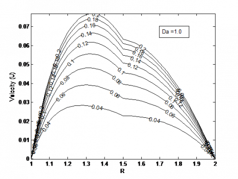
Figure 2 . Velocity profiles showing the effect of $\mathrm{Da}$ and $t(\gamma=0.5, d=1.5 \beta=-0.7, \lambda=2)$
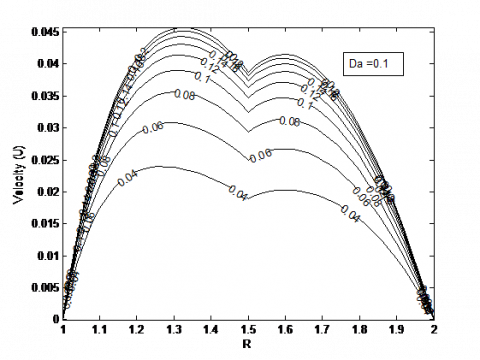
Figure 3. Velocity profiles showing the effect of Da and t (γ=0.5 , d=1.5 β=-0.7, λ=2)
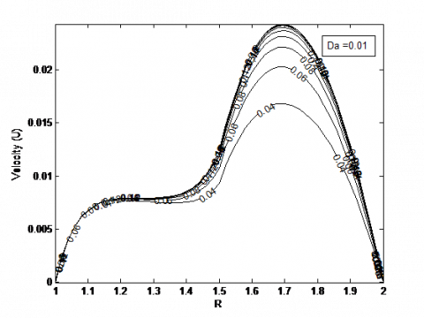
Variation of velocity profiles with time (t) and three different values of Darcy number (Da) 1.0, 0.1, 0.01 are presented in Figure 2, 3 and 4 respectively. In each case, its evident that velocity increases with increase in time (t) till it attains steady state velocity.
Figure 4. Velocity profiles showing the effect of Da and t (γ=0.5 , d=1.5 β=-0.7, λ=2)
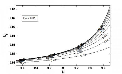
Figure 5. Interfacial velocity (Ui) for different values of β and t(γ=0.5 , d=1.5 , λ=2)
As Da becomes large, porous region is seen to be more permeable and greater fluid motion occurs in the porous region. The reverse trend occur for small a value of Darcy number (Da = 0.01) as velocity is seen to decrease sharply away from the fluids interface toward the outer surface of the inner cylinder due to less permeability of the porous region. Steady state velocity is reached faster for small value of Da while Large value of Da lengthen the time it takes to attain steady state velocity. This finding matches with the result of Jha and Odengle [16].
Figure 6. Interfacial velocity (Ui ) for different values of β and t (γ=0.5 , d=1.5 , λ=2)
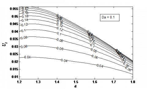
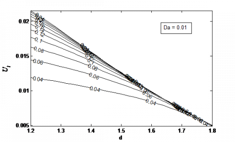
Figure 7. Interfacial velocity (Ui ) for different values of d and t (γ=0.5 , β=-0.7 , λ=2)
The combined influence of adjustable coefficient of the stress jump condition (β) and time (t) on interfacial velocity, Uiis reflected in Fig. 5 when Da=0.1. Ui is seen to be an increasing function of t and β till it attains steady state. A similar occurrence is observed in Fig. 6 when Da=0.01 with a sharp increase in velocity for large value of β. Both figures indicate that Ui decreases with increase in Da resulting in steady state been reached faster when $D a=0.01$ . This influence of time follows a similar trend as observed by Jha and Odengle [16 $]$ who did a similar analysis when the pressure gradient is applied in the axial direction. Figs. 7 and 8 depict the effect of time $(t)$ and interfacial radial distance $(d)$ on the interfacial velocity $U_{i}$ when $D a=0.1$ and 0.01 respectively. A steady increase in $U_{i}$ with $t$ is observed but decreases with $d,$ this is because as interfacial radial distance $d$ tends to $\lambda,$ the region occupied by fluid-saturated by porous material becomes large. Hence, high tendency for decrease in velocity resulting in a decrease in interfacial velocity.
Figure 8. Interfacial velocity $\left(U_{i}\right)$ for different values of $d$ and $t(\gamma=0.5, \beta=-0.7, \lambda=2)$
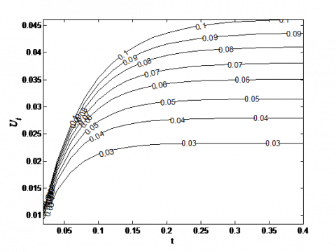
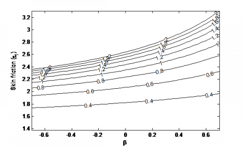
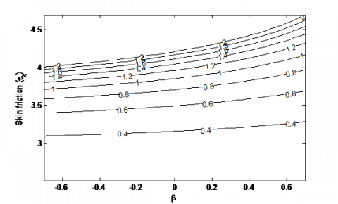
The reverse situation is obtained when d tends to the radius of the inner cylinder. The variation of $U_{i}$ with $D a$ and $t$ is presented in Fig. 9 . It is evident that $U_{i}$ increases with increase in $D a$ and $t .$ As $t$ comes large, a critical value of $t$ is reached when further increase in $t$ has no significant influence on $U_{i}$ . Fig. At this point, $U_{i}$ is said to be steady and independent of $t .$ Fig. 10 shows the effect of $\beta$ and $t$ on skin friction, $\tau_{1}$ (skinfriction at the outer surface of the inner cylinder R=1). At transient state, τ1 is seen to be an increasing function of β and t. further increase in $t$ has no impact on $\tau_{1} .$ similar occurrence is obtained in Fig. 11 as $\tau_{\lambda}$ (skin friction at the inner surface of the outer cylinder $R=\lambda )$ increases with increase $\beta$ and $t$ . It is noteworthy that $\tau_{1}$ is always less that $\tau_{\lambda},$ this is because thepresence of porous material at the porous region retards velocity hence, a decrease in magnitude of skin friction at that surface.
Figure 9. Interfacial velocity $\left(U_{i}\right)$ for different values of $D a$ and $t(\gamma=0.5, \beta=-0.7, \lambda=2)$
Figure 10 . Skin friction variation at the outer surface of the inner cylinder for different values of $\beta$ and $t(\gamma=0.5, d=1.5, D \mathrm{a}=0.1, \lambda=2 )$
Figure 11. Skin friction variation at the inner surface of the outer cylinder for different values of β and t (γ=0.5 , d=1.5 , Da=0.1, λ=2)
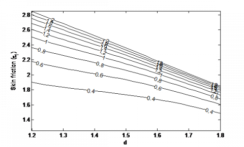
Figure 12 . Skin friction variation at the outer surface of the inner cylinder for different values of $d$ and $t(\gamma=0.5, \beta=-0.7, Da=0.1, \lambda=2 )$
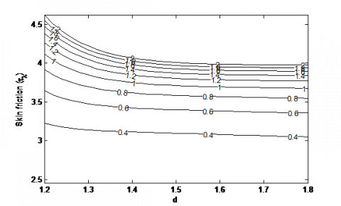
In Fig. $12,$ increase in $d$ suppresses $\tau_{1}$ since $\tau_{1}$ decreases with increase in d. $\tau_{1}$ also increases with $t$ till it attains steady state skin friction at the outer surface of the inner cylinder $(R=1) .$ Fig. 13 shows variation of $\tau_{\lambda}$ with respect to $d$ and $t .$ In a similar manner to Fig. $12, \tau_{\lambda}$ increases with $t$ till it reaches its steady state. It is noticed that $\tau_{\lambda}$ is fairly constant for a large value of $d$ . This indicates that decrease in the region occupied by clear fluid has no significant influence on skin friction at the inner surface of the outer cylinder. while an increase in the region filled by clear fluid increases $\tau_{\lambda}$ .
Figure 13 . Skin friction variation at the inner surface of the outer cylinder for different values of $d$ and $t(\gamma=0.5, \beta=-0.7, \lambda=2, D a=0.1 )$
With the explanation from Figs. 12 and $13,$ one can conclude that large value of $d$ (thin clear fluid region) increases $\tau_{1}$ but has no influence on $\tau_{\lambda}$ . While small value of $d$ (thin porous region) enhances skin friction at both surfaces. This is because high velocity of clear fluid always inspires skin friction at the surfaces.
The semi-analytical solution of the time dependent flow in an annulus partially filled with porous material due to sudden application of constant circumferential (Azimuthal) pressure gradient is considered. The annular gap is filled with a clear fluid and a fluid-saturated porous material of uniform permeability separated by a thin porous layer, with the clear fluid occuping the region near the inner surface of the outer cylinder. Laplace transform technique is used to solve the non-dimensional transport equations. The solution in Laplace domain is then inverted to time-domain using Riemann-sum approximation approach. In order to establish the accurary of the Riemann-sum approximation approach, a number of tables have been presented which shows that at large time, Riemann-sum approximation approach largely agrees with the steady state solution obtained exactly. To further demostrate reliability of this approach, a numerical scheme – the implicit finite defference is also used to solve the governing equations. The numerical values obtained from this two approaches (See table 1-4) indicates that they both match considerably at transient and steady state. The influence of a number of selected controlling parameters entering into the model is discused with the aid of line graphs. The main conclusions of the research work are
1. Generally, the unified velocity is an increasing function of time (t) till it attains steady state velocity.
2. A thin clear fluid region boosts τ1but has no influence on τλ. While thin porous region enhances skin friction at both surfaces.
3. There is a clear indication that porous region is more permeable with greater fluid motion arising in the porous region for a large value of Darcy number, this transitively enhanced the skin friction at the surfaces, The reverse trend occurs for a small value of Darcy number.
4. Positive value of β is observed to enhance interfacial velocity Ui, while large value of d (as d tends to the radii ratio) retards Ui. Furthermore, a linear relationship (See Fig. 8) is seen at steady state with negative gradient.
d Non-dimensional interfacial radial distance
d' Dimensional interfacial radial distance
Da Darcy number
I1 First-order modified Bessel function of the first kind
I2 Second-order modified Bessel function of the first kind
k' Permeability of the porous medium
K1 First-order modified Bessel function of the second kind
K2 Second-order modified Bessel function of the second kind
ri Radius of inner cylinder
ro Radius of outer cylinder
r' Dimensional radial coordinate
R Non-dimensional radial coordinate
t Time in non-dimensional form
t' Time in dimensional form
U non-dimensional velocity
u' dimensional velocity
Uo Reference velocity
Greek symbols
β Adjustable coefficient in the stress jump condition
γ Ratio of viscosity
λ Radii ratio
νeff Effective kinematic viscosity of the porous medium
ν Kinematic viscosity of the fluid
ρ Density
Subscripts
f Fluid region
i Interface between clear fluid and porous region
p Porous region
[1] Dean WR. (1928). Fluid motion in a curved channel. Proc. Roy. Soc. London A. 121: 402-420.
[2] Dryden HL, Murnaghan FD, Bateman H. (1956). Hydrodynamics. Dover Publ. Inc.
[3] Richardson EG, Tyler E. (1929). The transverse velocity gradient near the mouths of pipes in which an alternating flow is established. Proc. Phys. Soc. London. 42: 1-15.
[4] Gupta, RK, Gupta K. (1996). Steady flow of an elastico-viscous fluid in porous coaxial circular cylinder. Ind. J. Pure and Applied Math 27(4): 423-434.
[5] Samal RC, Biswal T. (2015). Fluctuating flow of a second order fluid between two coaxial circular pipes. IERT 4(2): 433-441.
[6] Drake DG. (1965). On the flow in a channel due to a periodic pressure gradient. Quart. J. of Mech. and Applied Math 18(1): 1-10.
[7] Fan C, Chao BT. (1965). Unsteady, laminar, incompressible flow through rectangular ducts. ZAMP 16(3): 1-360.
[8] Khamrui SR. (1957). The motion of the Newtonian fluids between two circular cylinders. Bull. Cal. Math. Soc. 49: 57.
[9] Haslam M, Zamir M. (1998). Pulsatile flow in tubes of elliptic cross sections. Ann. of Biomed. Eng. 26(5): 780-787.
[10] Tsangaris S. (1984). Oscillatory flow of an incompressible, viscous-fluid in a straight annular pipe. J. Mec. Theor. Appl. 3(3): 467.
[11] Tsangaris S, Vlachakis NW. (2007). Exact solution for the pulsating finite gap dean flow. Applied Mathematical Modelling 31: 1899-1906.
[12] Tsangaris S, Kondaxakis D, Vlachakis NW. (2006). Exact solution of the Navier–Stokes equations for the pulsating dean flow in a channel with porous walls. International Journal of Engineering Science 44: 1498-1509.
[13] Kuznetsov AV. (1997). Influence of the stress jump condition at the porous medium/clear fluid interface on a flow at a porous wall. Int. Comm. Heat Mass Transf. 24(3): 401-410. https://doi.org/10.1016/S0735-1933(97)00025-0
[14] Avramenko AA, Kuznetsov AV. (2009). Start-up flow in a channel or pipe occupied by a fluid-saturated porous medium. J. Porous Media 12(4): 361-367. https://doi.org/10.1615/JPorMedia.v12.i4.60
[15] Jha BK, Odengle JO. (2015). Unsteady Couette flow in a composite channel partially filled with porous material: a semi-analytical approach. Transp. Porous Med. 107: 219-234. https://doi.org/10.1007/s11242-014-0434-0
[16] Jha BK, Odengle JO. (2016). A semi-analytical solution for start-up flow in an annulus partially filled with porous material. Transp. Porous Med. 113(1). https://doi.org/10.1007/s11242-016-0724-9
[17] Paul T, Singh AK. (1998). Natural convection between coaxial vertical cylinders partially filled with a porous material. Forsch. Ing. (Eng. Res.) 64: 157-162. https://doi.org/10.1007/PL00010772
[18] Gibson RD, Cook AE. (1974). The stability of curved channel flow. Quart. J. Mech. Appl. Math. 27: 149-160. https://doi.org/10.1093/qjmam/27.2.149
[19] Deka RK, Gupta AS, Das SK. (2007). Stability of viscous flow driven by an azimuthal pressure gradient between two porous concentric cylinders with radial flow and a radial temperature gradient. Acta Mechanica 189: 73–86. https://doi.org/10.1007/s00707-006-0399-3
[20] Andersson HI, Tiseth KL. (1992). Start-up flow in a pipe following the sudden imposition of a constant flow rate. Chem. Eng. Commun. 112(1): 121-133. https://doi.org/10.1080/00986449208935996
[21] Kataoka K, Kawabata T, Miki K. (1975). The start-up response of pipe flow to a step change in flow rate. J. Chem. Eng. Japan 8: 266. https://doi.org/10.1252/jcej.8.266
[22] Gupta S, Poulikakos D, Kurtcuoglua V. (2008). Analytical solution for pulsatile viscous flow in a straight elliptic annulus and application to the motion of the cerebrospinal fluid. Physics of Fluids 20: 093607. https://doi.org/10.1063/1.2988858
[23] Mishra SP, Roy JS. (1968). Flow of elastico-viscous liquid between rotating cylinders with suction and injection. Physics of Fluids 11(10): 2074-2081. https://doi.org/10.1063/1.1691786
[24] Chikh S, Boumedien A, Bouhadef K, Lauriat G. (1995). Non-Darcian forced convection analysis in an annulus partially filled with a porous material. Numer. Heat Transf. A 28(6): 707-722. https://doi.org/10.1080/10407789508913770
[25] Chikh S, Boumedien A, Bouhadef K, Lauriat G. (1995). Analytical solution of non-Darcian forced convection in an annular duct partially filled with a porous medium. Int. J. Heat Mass Transf. 38(9): 1543-1551. https://doi.org/10.1016/0017-9310(94)00295-7
[26] Chandrasekhar S. (1960). The hydrodynamic stability of viscid flow between coaxial cylinders. Proc. N.A.S. 46: 137-141.
[27] Rajgopal KR, Na TY, Gupta S. (1985). Flow of a viscoelastic fluid between two coaxial cylinders. Rerol. Acta. 23: 213-215.
[28] Biswal T, Mishra BK. (1985). Fluctuating flow of viscoelastic liquid between two coaxial cylinders. Rev. Roum. Phys. Tome 30(7): 573-578.
[29] Qi H, Jin H. (2006). Unsteady rotating flows of a viscoelastic fluid with the fractional Maxwell model between coaxial cylinders. Acta. Mech. Sinia. 22(4): 301-305. https://doi.org/10.1007/s10409-006-0013-x
[30] Nazar M, Fetecau C, Awan AU. (2010). A note on the unsteady flow of a generalized second grade fluid through a cylinder subject to time dependent shear stress. Nonlinear Anal.: Real World App. 11: 2207-2214.
[31] Jha BK, Yusuf TS. (2016). Transient free convective flow in an annular porous medium: A semi-analytical approach. Eng. Sci. and Tech. An Int. J. 19: 1936–1948. https://doi.org/10.1016/j.jestch.2016.09.022
[32] Jha BK, Apere CA. (2011). Unsteady MHD two-phase Couette flow of fluid–particle suspension in an annulus. AIP Adv. 1: 042121-1–042121-15. https://doi.org/10.1063/1.3657509
[33] Khadrawi AF, Al-Nimr MA. (2007). Unsteady natural convection fluid flow in a vertical microchannel under the effect of the Dual-Phase-Lag heat conduction model. Int. J. Thermophys. 28: 1387–1400. https://doi.org/10.1007/s10765-007-0207-x
[34] Tzou DY. (1997). Macro to Microscale Heat Transfer: The Lagging Behavior, Taylor and Francis, London.