Simplified analysis of heat transfer through a finned tube bundle in air cooled condenser

2.1 Transverse crossing of a finned tube. Local variation of Nusselt number

In general, transverse batting of solitary cylinders (or a package of these) results in flow separation, which is difficult to handle analytically. Therefore, flows of this type should be studied experimentally or numerically. In fact, flow through cylinders and cylinder packs has been studied experimentally by numerous researchers and several empirical correlations have been developed for the determination of heat transfer coefficient [6-8]. The complicated pattern of the flow through a single finned cylinder greatly influences the heat transfer.

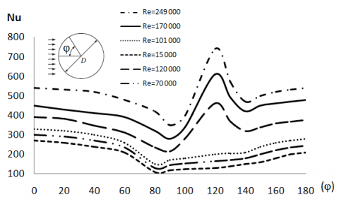
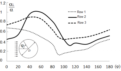
Many investigations have been carried out in order to clarify this problem. In figure 1 are given the average values of the experimental results reported by [2-3]. This figure provides the variation of the local Nusselt number $\mathrm{V} u$ depending on the angle $\varphi$ , on the periphery of a finned cylinder bathed by a cross and perpendicular airflow.

A detailed analysis of figure 1 and the available experimental quantities allows us to establish that in the transversal bathing of a cylinder finned by a turbulent airflow, two basic regions are formed depending on the dimensionless number of. The first in the interval $4 \cdot 10^{3} \leq \operatorname{Re} \leq 10^{5}$  and the second in $10^{5}<\operatorname{Re} \leq 4 \cdot 10^{5}$ .

In the first interval the value of $N u$  starts relatively high at the stagnation point $\left(\varphi=0^{\circ}\right)$ , reaching at this point its maximum value $\left(N u_{M A Y}\right)$ . For $0^{0}<\varphi \approx 60^{\circ}$ , $N u$  presents a decreasing tendency very close to a linear function with negative slope $m \approx-1.15$ . In interval $60^{\circ}<\varphi \approx 80^{\circ}$  the downward trend undergoes a sharp change in slope taking now $-5<m \approx-6$ . In both cases this decrease is caused by the thickening of the laminar boundary layer.

In the point $\varphi \approx 80^{\circ}$ separation of the laminar flow occurs, and therefore it is logical that the number of $\mathrm{N} u$  reach its minimum value, causing this to also coincide in $\varphi \approx 80^{\circ}$  the presence of a positive inflection point. At this point it is true that $N u \approx\left(N u_{M \ell X}\right)^{0.84}$ , For $80^{\circ}<\varphi \leq 180^{\circ}$ , $N u$ present a clear tendency to grow as a result of intense mixing in the region of the separate stream (the wake). This growth follows approximately a positive slope line $m \approx 1.15$ until $\varphi \approx 180^{\circ}$ .where it is true that $N u \approx 0.9 \mathrm{Nu}_{\mathrm{MAX}}$ .

However the second region $10^{5}<\mathrm{Re} \leq 4 \cdot 10^{5}$  its behavior differs from the first. In the first interval, value of $N u$  starts relatively high at the point of stagnation $\left(\varphi=0^{\circ}\right)$ , reaching at this point a high value. $\left(N u_{0}\right)$  but not maximum as happened in the first region. For $0^{0}<\varphi \approx 90^{\circ} \mathrm{N} u$ number present a decreasing tendency very close to a linear function with negative slope $m \approx-1.8$ . The point $\varphi \approx 90^{\circ}$  is where the laminar flow separation occurs, and therefore it is logical that the Nusselt number reaches its minimum value and this point is at once an inflection point. At this point it is true that $N u \approx\left(N u_{0}\right)^{0.92}$ .

For $90^{\circ}<\varphi \leq 120^{\circ}$ , $N u$ number present a clear tendency to growth being asymptotically guided by a positive slope whose value varies in the intervals. 12$\approx m \approx 14$ . This increase in the local number is due to the transition from laminar to turbulent. In $\varphi=120^{\circ}$  is where a maximum $\left(N u_{M A Y}\right)$  and a second point of inflection are located, what is fulfilled $N u_{M A X}=\left(N u_{0}\right)^{1.05}$ .

For the $N u$ number present a pronounced decreasing behavior, not ruled by a single slope, until reaching $\varphi \approx 140^{\circ}$ , at which point the second minimum of the local $N u$ number is presented, being fulfilled that $N u=\left(N u_{0}\right)^{0.98}$ .

This point is precisely where the separation of the flow occurs in the turbulent flow. For $140^{\circ}<\varphi \leq 180^{\circ}$ , a new growth of the local number as a result of the intense mixing in the turbulent region of the wake, this growth presents an asymptotic behavior to a linear function with a positive slope that oscillates in the interval 4.1$\approx m \approx 4.8$ , is also fulfilled in that, $\varphi=180^{\circ}$  that $N u=(16 / 15) \cdot\left(N u_{0}\right)$ .

The discussions given in the previous paragraphs about the local heat transfer coefficients provide insight into the behavior of this at any point in the finned cylinder and for any operant flow regime, however, have little value in the transfer calculations of heat, since in these the average heat transfer coefficient over the entire surface is required. The main author provides a detailed discussion of this problem in the reference [10].

1.png

Figure 1. Local Nusselt number variation as a function of the angle in air cross flow over finned cylinder

2.2 Transverse crossing of a bundle of finned tubes

The tubes bank is usually arranged in a row or triangle in the direction of flow, as shown in Figure 2. The outside tube diameter is taken as the characteristic length. The arrangement of the tubes in the bench is characterized by the transverse passage S_T. the longitudinal passage S_L and the diagonal step S_D between the centers of the tubes (see figure 2).

The diagonal step is determined from the following equation:

$S_{D}=\sqrt{S_{L}^{2}+\left(\frac{S_{T}}{2}\right)^{2}}$              (1)

As the fluid enters the bank, the flow area decreases from $A_{T}=S_{T} L$ to $A_{T}=\left(S_{T}-d\right) L$  between the tubes, and as a consequence, the flow velocity increases [17]. In the stepped arrangement the speed can increase further in the diagonal region if the rows of tubes are very close together. In tube banks, the characteristics of the flow are dominated by the maximum velocity $V_{M \alpha x}$ , which is held within the bank, rather than by the approximate velocity V. Therefore, the Reynolds number is defined on the basis of the maximum velocity as:

$\operatorname{Re}_{d}=\frac{\rho V_{\operatorname{Max}} d}{\mu}=\frac{V_{\operatorname{Max}} d}{v}$            (2)

The maximum velocity is determined based on the mass conservation requirement for the incompressible stationary flow. For alignment arrangement, the maximum velocity is in the minimum flow area between the tubes and the mass conservation can be expressed as (see Figure 2):

$\rho V A_{1}=\rho V_{M C \alpha} A_{T}=V_{M \alpha x}\left(S_{T}-d\right)$             (3)

Then from Equation (3) it follows that the maximum velocity will be as:

$V_{M c x}=\frac{S_{T}}{S_{T}-d} V$              (4)

In the stepwise arrangement the fluid approaching through the area A₁ (See Figure 2) passes through the area A_T and before for area 2A_D, as it is wound around the tube in the next row. If it is true that 2A_D > A_T, the maximum speed still occurs in A_T between the tubes and consequently, the V_Max in Equation (4) can be used for staggered bundles tube.

2.png

Figure 2. Tubes arrangement in a bank

If it happened that $2 A_{D}<A_{T}\left[\text { that is if } 2\left(S_{D}-d\right)<\left(S_{T}-d\right)\right]$, the maximum velocity will be taken in the diagonal cross-sections and. in this case, that maximum velocity is given by:

$V_{M \alpha x}=\frac{S_{T}}{2\left(S_{D}-d\right)} V$          (5)

The conservation of mass can be expressed as (see Figure 2):

$\rho V A_{1}=\rho V_{M \alpha x}\left(2 A_{D}\right)$           (5.1)

Or what is the same.

$V S_{T}=2 V_{M \alpha x}\left(S_{D}-d\right)$           (5.2)

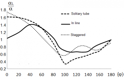
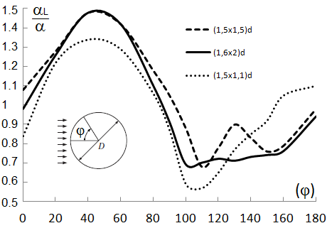
The peculiarities of heat transfer in the transverse flow in a tube bank are very similar to those found in a solitary tube. The variation of heat transfer around a tube bank is determined by the flow pattern, which depends largely on the arrangement of the tubes. Thus in line layout banks, there are two collision points, which results in two thermal transfer peaks. However in banks with staggered arrangement, the process of heat transfer is to some extent similar to that of a solitary tube. Figure 3 provides a comparison of the quotient arising between the local heat transfer coefficient and the average heat transfer coefficient for a solitary tube and for the third row of in-line and stepped arrangements.

Local heat transfer coefficients plotted in Figure 3 correspond to the average value of a measurable group of measurements reported in [2, 11] for $\mathrm{Re}=7 \cdot 10^{4}$ and arrangements $(1,5 x 2) D$ , that is, the transverse passage $S_{T}=1.5 \cdot D$ and the longitudinal passage $S_{L}=2 \cdot D$ .

Figure 3 shows that in the aligned arrays the maximum local heat transfer is located at the point $\varphi=50^{\circ}$ , while the stepped arrangement has two maxima, one at the point of fluid stagnation $\varphi=0^{0}$ and another in the separation of the flow in. It is expected that the presence of two maxima will cause the area under the curve to be larger in the staggered arrangements and therefore, taking into account also the low corrosion and deposition properties of the air, make preferable the stepped arrangement for ACC systems, because with this a higher average heat transfer coefficient is achieved. An inspection of ACC manufacturer’s catalogs confirms that the staggered arrangement is the one used in all marketed equipment.

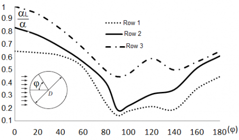
In any type of arrangement the heat transfer coefficient increases from the first row of tubes to the third, and takes a constant value from the latter. In figure 4 and 5 are plotted for staggered and in-line arrangements, respectively, the average experimental values reported by the authors [9] for the first three rows of a tube package of an ACC. for $\mathrm{Re}=1.4 \cdot 10^{4}$ and one dimension $(2 \times 2) D$ .

The row variation in aligned arrangements does not produce significant changes in local heat transfer coefficient. The authors [8-11], who examined experimentally arrangements with different dimensions, confirm this criterion and for a fixed value of $\operatorname{Re}=3 \cdot 10^{4}$ .The, results obtained confirm that the local heat transfer coefficient follows approximately a common pattern for all the arrangements examined. In figure 6 are plotted the averages available values.

An analysis of 738 sets of available experimental data, reported by 10 authors linked to centers of high prestige [13-15], allowed developing a dimensionally non-homogeneous expression, which was generated by an integral analysis of residues by cross-methods of breaks at intervals, describing with a mean error of the order $\pm 6.5 \%$  in the 84.8% of the available experimental samples.

This equation is given by the following expression:

$\alpha=\frac{\left(T_{T B S}\right)^{0.0064}\left(V_{\max }\right)^{0,6}(e \cdot h)^{0.01}}{\left[0.15\left(S_{T}-d\right)^{0,4}\right] \cdot 0.17 \operatorname{Ln}(F)}\left(\mathrm{W} / \mathrm{m}^{2} \mathrm{K}\right)$           (6)

In Equation (6):

$T_{T B S}$ is the dry bulb temperature, in ⁰C

$V_{\max }$ is the velocity in the narrowest section of the tube package, in m/s

$e$ is the fins thickness , in mm

$h$ is the fins height, in mm

$F$ is the number of fins per linear meter in length of the finned tube.

The value of $V_{m}$ is determined by the use of the following relations:

if $\quad 2\left(S_{D}-d\right)>\left(S_{T}-d\right) \quad ; \quad V m=\frac{S_{T}}{S_{T}-d} V_{0}$

if $\quad 2\left(S_{D}-d\right) \leq\left(S_{T}-d\right) \quad ; \quad V m=\frac{S_{T}}{2\left(S_{D}-d\right)} V_{0}$          (7)

While the diagonal step is given by:

$S_{D}=\sqrt{S_{L}^{2}+\left(\frac{S_{T}}{2}\right)^{2}}$(m)              (8)

where:

$V_{0}$  It is the airflow velocity at entry to the finned tube pack, in m/s

$S_{T}$ is the transverse step, in m

$S_{L}$ is the longitudinal step, in m

$S_{D}$ is the diagonal step, in m

D is the external diameter of the tubes + fins, in m

d is the outer diameter of the bare tubes (without fins), in m

3.png

Figure 3. Local heat transfer coefficient variation for different arrangements of finned tubes

4.png

Figure 4. Variation of a local heat transfer coefficient in ACC with staggered arrangement

Expression (6) is valid for $15 \leq T_{T B S} \leq 43^{\circ} C$ , for a refrigerant speed between 0.1 and 20 m/s, as well as ratios $0.4<S_{T} / S_{L}<2$ ,external diameters of plain tubes $0.019<d<0.035 m$ ,a wind velocity incident on installation between 0 and 45 km/h, a height of the fins between 2.7 and 7.5 mm, thicknesses of the fins ranging between 2.3 and 3 mm and a number of fins per unit of pipe length between 315 and 394.

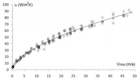
A total of 738 sets of available experimental data found a mean error of the order $\pm 6.5 \%$  to the 84.8% of the correlated experimental samples. Table 1 provides a summary of the main parameters of the experimental quantities available and the mean deviation values found in each case. Figure 7 gives the correlation of available experimental samples with Equation (6).

5.png

Figure 5. Variation of a local heat transfer coefficient in ACC with aligned arrangement

6.png

Figure 6. Local heat transfer coefficient variation for different dimensions in ACC with aligned arrangement

7.png

Figure 7. Correlation of available experimental samples with equation (6)

Table 1. Comparison between Equation (6) and experimental values available for staggered arrangements in ACC systems

This work was supported by Doctoral Research Program of Universidad Central “Marta Abreu” de las Villas, Cuba.