OPEN ACCESS
The aim of study is to analyse steady two dimensional laminar, boundary layer flow of incompressible, viscous nanofluid with MHD along with heat generation and suction effect is considered. This problem is of wide importance in importance. Two types of nanofluids namely silver and Titanium oxides with water as base fluid are considered. Partial differential equations are converted into ordinary differential equations using similarity transformation. Differential equations are solved using HAM (Homotomy Analysis Method). Effect of various physical parameters on temperature and velocity profile is investigated with help of graphs. Values of skin friction coefficient and rate of heat transfer are also tabulated. The results hold good agreement with previous works. The result has great contribution in extrusion of polymers.
nanofluids, inclined stretching sheet, HAM, MHD
Nanofluids are special type of fluids consisting of base fluid with small nanosized particle (1- 10 nm) suspended in them. They were first introduced by Choi⦋1⦌. Water, ethylene glycol is widely used as base fluid. Nanoparticles may be metals (Al, Cu, Ag, Au, Fe), their oxides (Al2O3, CuO, TiO2), their carbide, (SiC), Nitride (AlN,SiN ) or even non metals (graphite carbon nanotubes). Due to enhancement in thermophysical properties nanofluids have gained wide interest in recent years. It was proved experimentally that by increasing 1-5 % volume fraction of nanoparticles, the thermal conductivity increases by 20%. Buogiorno ⦋4⦌ explained significant increase in thermal conductivity.
Nanofluids can be widely used in industries, cooling devices like vehicle cooling, transfer cooling, electronic cooling. They are effectively used by cooling, medical fields like safer surgery by cooling.
Many researchers have worked on boundary layer flow along with heat transfer over a stretching sheet due to its tremendous application in field of engineering and industry. Industrial processes like drawing continuous filament and fibre spinning, extrusion of polymer, glass fibre production. During the process of manufacturing these sheets, metal is stretched to achieve desired thickness. The final product depends upon rate of cooling and stretching rate. This can be done by using an electrically conducting fluids and applying MHD. Khan and Pop ⦋1⦌ discussed boundary layer flow of nanofluids over a stretching sheet and investigated it numerically.
Almost all equations related to scientific problem and industrial application are nonlinear in nature. Very few of them may have exact solution. Liao ⦋23,24⦌ gave a new technique for solving nonlinear ordinary as well as partial differential equation known as homotopy analysis method (HAM). It is semi analytical method to get solution of strongly nonlinear equations. It ensures convergence of solution in series.
The main aim of our study is to find a better coolant. It also indicates that silver nanofluid is better nanoparticle than any other nanoparticle which are commonly used like copper. This paper has contribution in field of cooling process of tools and equipment. This study can be extended to hybrid nanofluid.
In present study, we analyze effects of internal heat generation over mixed convective hydro magnetic flow over a stretching sheet for silver water nanofluids. The partial differential equations are reduced to ordinary differential equations using similarity transformation. These ODE’s are then solved by HAM. The effect of various parameters like magnetic parameters, suction parameters, mixed convection parameters, angle of inclination parameters etc. are depicted with help of suitable graph.
Let us consider two dimensional steady flow of incompressible and electronic conducting nano fluid past over a linear stretching sheet inclined at an angle α to the vertical direction. Velocity of stretching sheet is taken as u = ax; where is a constant and a>0. The temperature of stretching sheet is taken Tw(x) = T∞+bx.
Direction along the sheet is taken as X axis and Y axis perpendicular to it. We have two equal and opposite force on the stretching sheet. A uniform magnetic field of strength B0 is applied normally to the sheet i.e. along Y axis. Suction velocity vwis normal to the sheet. Following assumptions are made:
Equations of conservation of mass, energy and momentum as given by Prandtl are as follows:
$\frac{\partial u}{\partial x}+\frac{\partial v}{\partial y}=0$ (1)
$u \frac{\partial u}{\partial x}+v \frac{\partial u}{\partial y}=v \frac{\partial^{2} u}{\partial y^{2}}+\frac{g(\rho \beta)_{n f}\left(T-T_{\infty}\right)}{\rho_{n f}} \cos \alpha-\frac{\sigma B_{0}^{2} u}{\rho_{n f}}$ (2)
$u \frac{\partial T}{\partial x}+v \frac{\partial T}{\partial y}=\alpha_{n f} \frac{\partial^{2} T}{\partial y^{2}}+\frac{Q_{0}\left(T-T_{\infty}\right)}{\left(\rho c_{p}\right)_{n f}}$ (3)
Along with boundary condition:
$\mathrm{y}=0, \mathrm{u}=\operatorname{Uw}(\mathrm{x})=\mathrm{ax}$ $y \rightarrow \infty, u \rightarrow 0, T \rightarrow T_{\infty}$ (4)
The density specific heat and heat capacitance of nanofluid:
$\rho_{n f}=(1-\emptyset) \rho_{f}+\phi \rho_{S}$ (5)
$\left(\rho C_{p}\right)_{n f=(1-\emptyset)\left(\rho c_{p}\right)_{f}}+\emptyset\left(\rho C_{p}\right)_{s}$ (6)
$(\rho \beta)_{n f}=(1-\phi)(\rho \beta)_{f}+\phi(\rho \beta)_{s}$ (7)
The dynamic viscosity of nanofluid as formulated by Brickman:
$\mu=\frac{\mu_{f}}{(1-\emptyset)^{2.5}}$ (8)
The ratio of thermal conductivity of spherical shaped nanofluids to that of base fluid is given by Maxwell Garnett’s model:
$\frac{k_{n f}}{K_{f}}=\frac{\left(k_{s}+2 k_{f}\right)-2 \emptyset\left(k_{f}-k_{s}\right)}{\left(k_{s}+2 k_{f}\right)+\emptyset\left(k_{f}-k_{s}\right)}$ (9)
Thermal diffusibilty of nanofluid is given by:
$\alpha_{n f}=\frac{k_{n f}}{\left(C_{p}\right)_{n f}}$ (10)
|
|
ρ(kg/m3) |
β(k-1) |
k(W/m.k) |
Cp(J/kg.k) |
|
Water |
997.1 |
21x10-5 |
0.613 |
4179 |
|
Silver |
10,500 |
1.89x10⁻⁵ |
429 |
235 |
|
Titanium oxide |
4250 |
0.9x10⁻⁵ |
8.9538 |
686.2 |
P.D.E are converted into ODE using similarity variable $\eta$.
$\psi=\left(a \vartheta_{n f}\right)^{1 / 2} x f(\eta)$ (11)
$\eta=\left(\frac{a}{\vartheta_{n f}}\right)^{1 / 2} y$ (12)
$u=a x f^{\prime}(\eta)$ (13)
$v=-\left(a \vartheta_{n f}\right)^{\frac{1}{2}} f(\eta)$ (14)
where ψ(x, y) is stream function and $u=\frac{\partial \psi}{\partial y} \operatorname{and} v=-\frac{\partial \psi}{\partial x}$ and,
$\theta(\eta)=\frac{T-T_{\infty}}{T_{W}-T_{\infty}}$ (15)
Equations (2) and (3) are transformed into ordinary differential equation given below:
$f^{\prime \prime \prime}+(1-\emptyset)^{2.5}\left\{\left(f f^{\prime \prime}-f^{\prime 2}\right)\left(1-\emptyset+\emptyset \frac{\rho_{s}}{\rho_{f}}\right)-M^{2} f^{\prime}+\lambda \theta\left(1-\emptyset+\emptyset \frac{(\rho \beta)_{s}}{(\rho \beta)_{f}}\right) \cos \alpha\right\}=0$ (16)
$\frac{1}{\operatorname{Pr}_{n f}} \frac{k_{n f}}{k_{f}} \theta^{\prime \prime}+\left(1-\emptyset+\emptyset \frac{\left(\rho c_{p}\right)_{s}}{\left(\rho c_{p}\right)_{f}}\right)\left(f \theta^{\prime}-f^{\prime} \theta\right)+\beta_{1} \theta=0$ (17)
Along with boundary conditions:
At $\eta=0, \quad f=S, f^{\prime}=1, \theta=1$ As $\eta \rightarrow \infty, \quad f^{\prime} \rightarrow 0, \theta \rightarrow 0$ (18)
where $k=l\left(\frac{a}{\vartheta}\right)^{1 / 2} ; \mathrm{S}=\frac{v_{w}}{\left(a \vartheta_{f}\right)^{1 / 2}}$ denotes differentiation w.r.t. η.
Terms used in equation are:
$(\operatorname{Rex})_{f}=\frac{U_{w} x}{\vartheta_{f}} ; c=\frac{g \beta\left(T_{w}-T_{\infty}\right) x^{3}}{\vartheta_{f}^{2}} ; \lambda=\frac{g \beta\left(T_{w}-T_{\infty}\right)}{a^{2} x}$ $\operatorname{Pr}=\frac{\vartheta_{f}}{\alpha_{f}} ; M^{2}=\frac{\sigma B_{0}^{2}}{a \rho_{f}} ; A=\frac{v_{w}}{\left(a \vartheta_{f}\right)^{1 / 2}} ; \beta_{1}=\frac{Q_{0}}{a\left(\rho c_{p}\right)_{f}}$
where $(Rex)_{f}$ is local Reynold's number; $(Grx)_{f}$ is Grashouf number; λ is mixed convection parameter; Pr is Prandtl number; M2 is magnetic parameter; A is suction parameter; β1 is heat source parameter.
2.2 Nusselt number
Nusselt number is defined by:
Using (15) we get
$N u R e_{x}^{-1 / 2}=-\frac{k_{n f}}{K_{f}} \theta^{\prime}(0)$
2.3 Solution by means of HAM
As per boundary conditions and solution given by Liao
$f(\eta)=f_{0}(\eta)+\sum_{i=1}^{\infty} f_{i}(\eta)$ $\theta(\eta)=\theta_{0}(\eta)+\sum_{i=1}^{\infty} \theta_{i}(\eta)$
where $f_{0}(\eta)=S+1-e^{-\eta}, \theta_{0}(\eta)=e^{-\eta}$
where auxiliary linear operator are given by
which satisfies conditions
$L_{f}\left[c_{1}+c_{2} e^{\eta}+c_{3} e^{-\eta}\right]=0$ $L_{\theta}\left[c_{4} e^{\eta}+c_{5} e^{-\eta}\right]=0$
where ci (i= 0,1,2….5) are constants.
Nonlinear operators are defined:
$N_{1}[\hat{f}(n ; p) ; \hat{\theta}(n ; p)]=\frac{\partial^{3} \hat{f}(n ; p)}{\partial \eta^{3}}+(1-\phi)^{2.5}$
$\left\{\left(\hat{f}(n ; p) \frac{\partial^{2} \hat{f}(n ; p)}{\partial \eta^{2}}-\frac{\partial \hat{f}(\eta ; p)^{2}}{\partial \eta}\right) \left(1-\Phi+\Phi \frac{\rho_{s}}{\rho_{f}}\right) +M^{2} \frac{\partial \hat{f}(\eta ; p)}{\partial \eta}+\lambda \widehat{\theta}(\eta ; p) \left(1-\phi+\phi \frac{(\rho \beta)_{s}}{(\rho \beta)_{f}} \cos \alpha\right) \right\}=0$
$N_{2}[\hat{f}(n ; p) ; \hat{\theta}(n ; p)]=\frac{1}{\operatorname{Pr}} \frac{k_{n f}}{k_{f}} \frac{\partial^{2} \overline{\theta}(n ; p)}{\partial \eta^{2}}+\left[(1-\phi)+\Phi \frac{\left(\rho_{C p}\right)_{s}}{\left(\rho_{C p}\right)_{f}}\right]$ $\left(\hat{f}(n ; p) \frac{\partial \widehat{\theta}(\eta ; p)}{\partial \eta}-\frac{\partial \hat{f}(\eta ; p)}{\partial \eta} \hat{\theta}(n ; p)\right)+H_{s} \hat{\theta}(n ; p)$
where $p \in[0,1]$ is embedding parameter and $\hat{f}(n ; p)$ and $\widehat{\theta}(n ; p)$ are type of mapping functions.
Zero order deformation equations are
$f_{m}(\eta)=\frac{1}{m !} \frac{\partial^{m} \hat{f}(\eta ; p)}{\partial p^{m}}$
And
$\theta_{m}(\eta)=\frac{1}{m !} \frac{\partial^{m} \widehat{\theta}(\eta ; p)}{\partial p^{m}}$ at $\mathrm{p}=0$
The mth order deformation equation are:
$L_{f}\left[f_{m}(\eta, p)-\chi_{m} f_{m-1}(\eta)\right]=h R_{m}^{f}(\eta)$
$L_{\theta}\left[\theta_{m}(\eta, p)-\chi_{m} \theta_{m-1}(\eta)\right]=h R_{m}^{\theta}(\eta)$
where
where
The general solution is given by
$f_{m}(\eta)=f_{m}^{*}(\eta)+c_{1}^{m}+c_{2}^{m} \eta+c_{3}^{m} e^{-\eta}$
$\theta_{m}(\eta)=\theta_{m}^{*}(\eta)+c_{4} e^{\eta}+c_{5} e^{-\eta}$
Laminar flow of two nanofluids over an inclined stretching sheet is studied with mixed convection. The non-linear differential equations with the boundary conditions were solved with the help of HAM. The Homotopy Analysis Method (HAM) is very efficient method to solve highly nonlinear equation. Stability analysis for fluid flow is done. The Prandtl number is considered as 6.2 and mixed convection parameter is taken as 1.5. In absence of volume fraction, suction parameter result shows good agreement with Ishak et. al.
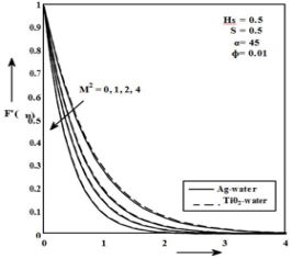
Figure 1. Dimensionless velocity profiles for different M2
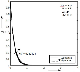
Figure 2. Temperature distribution for different M2
Figure 3. Dimensionless velocity profiles for different α
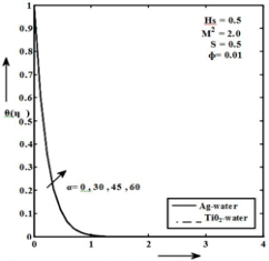
Figure 4. Temperature distribution for different α
Various physical parameters like M2, α, ф, S are calculated. Stability analysis is done. Some of inferences drawn from graph are as follows:
Figure 1 shows effect of magnetic parameter over dimensionless velocity for nanofluids. Due to magnetic field Lorentz force is induced which results in decrease of velocity i.e. increase in magnetic field results in decrease in velocity. Effect of magnetic field on temperature profile is depicted in figure 2. It was found that increasing value of magnetic field increases temperature. Thermal boundary layer thickness increases due to increase in magnetic field.
Figure 3 displays value of α on velocity profile. It was observed that as angle increases velocity decreases. Figure 4 depicts the effect of angle inclination of stretching sheet on dimensionless temperature. Increase in angle leads to increase in temperature.
Figure 5. Dimensionless velocity profiles for different Hs
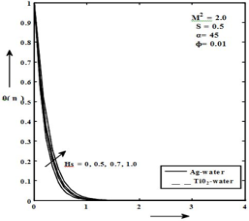
Figure 6. Temperature distribution for different Hs
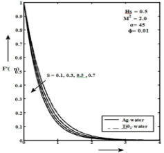
Figure 7. Dimensionless velocity profiles for different S
Figure 8. Temperature distribution for different S
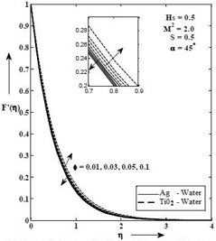
Figure 9. Dimensionless velocity profiles for different φ
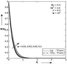
Figure10. Temperature distribution for different
Figure 5 shows the impact of heat generation parameter on velocity profile. Increase in heat generation results in increase in buoyant force which leads to increase in velocity. Thermal boundary layer thickness of nanofluid increases with heat generation parameter. Figure 6 depicts effect of heat generation parameter on temperature. It is obvious that increase in heat generation parameter increases thermal state. It was concluded that thermal boundary layer thickness increases due to increase in heat generation parameter.
Table 2. Skin friction coefficient for silver water and titanium oxide nanofluids
|
Ф |
M2 |
A |
K |
A |
β1 |
$\mathbf{A} \mathbf{g} \frac{\mathbf{1}}{(\mathbf{1}-\emptyset)^{2.5}} \boldsymbol{f}^{\prime \prime}(\mathbf{0})$ |
$\operatorname{Ti} \mathrm{O}_{2}\frac{1}{(1-\phi)^{2.5}} f^{\prime \prime}(0)$ |
|
0.01 0.03 0.05 0.1 |
2 |
450 |
0.1 |
0.5 |
0.5 |
-1.882491 -2.019789 -2.149876 -2.492271 |
-1.866731 -1.940001 -2.018998 -2.221124 |
|
0.01 |
0 1 2 4 |
450 |
0.1 |
0.5 |
0.5 |
-1.176284 -1.569889 -1.882491 -2.391517 |
-1.1389967 -1.539929 -1.866731 -2.376892 |
|
0.01 |
2 |
00 300 450 600 |
0.1 |
0.5 |
0.5 |
-1.823112 -1.855624 -1.882491 -1.939989 |
-1.785437 -1.824268 -1.866731 -1.915930 |
|
0.01 |
2 |
450 |
0 0.1 0.2 0.3 |
0.5 |
0.5 |
-1.678921 -1.882491 -2.011729 -2.034671 |
-1.658941 -1.866731 -2.009729 -2.02346 |
|
0.01 |
2 |
450 |
0.1 |
0.1 0.3 0.5 0.7 |
0.5 |
-1.586177 -1.736721 -1.872491 -2.037892 |
-1.576891 -1.732912 -1.866731 -2.037892 |
|
0.01 |
2 |
450 |
0.1 |
0.5 |
0.0 0.5 0.7 1.0 |
-1.906789 -1.882491 -1.876542 -1.869212 |
-1.870999 -1.866731 -1.849937 -1.836392 |
Table 3. Rate of heat transfer for silver water and titanium oxide nanofluids for various parameters (taking λ=1.5 and Pr=6.2)
|
Ф |
M2 |
α |
K |
A |
β1 |
$\mathbf{A} \mathbf{g}\left(-\frac{\boldsymbol{k}_{n f}}{\boldsymbol{K}_{f}} \boldsymbol{\theta}^{\prime}(\boldsymbol{0})\right)$ |
$\mathbf{T} \mathbf{i} \mathbf{O}_{2}\left(-\frac{\boldsymbol{k}_{n f}}{\boldsymbol{K}_{f}} \boldsymbol{\theta}^{\prime}(\mathbf{0})\right)$ |
|
0.01 0.03 0.05 0.1 |
2 |
450 |
0.1 |
0.5 |
0.5 |
4.352261 4.365769 4.380012 4.408958 |
4.351628 4.369065 4.384122 4.429125 |
|
0.01 |
0 1 2 4 |
450 |
0.1 |
0.5 |
0.5 |
4.516251 4.423689 4.352261 4.237845 |
4.364127 4.358602 4.351628 4.237904 |
|
0.01 |
2 |
00 300 450 600 |
0.1 |
0.5 |
0.5 |
4.362131 4.358299 4.352261 4.345163 |
4.364719 4.358710 4.351628 4.100378 |
|
0.01 |
2 |
450 |
0 0.1 0.2 0.3 |
0.5 |
0.5 |
4.607891 4.352261 4.201789 4.109981 |
4.606789 4.351628 4.200021 4.100378 |
|
0.01 |
2 |
450 |
0.1 |
0.1 0.3 0.5 0.7 |
0.5 |
2.421512 3.349972 4.352261 5.427891 |
2.421780 3.348169 4.351628 5.412010 |
|
0.01 |
2 |
450 |
0.1 |
0.5 |
0.0 0.5 0.7 1.0 |
4.885642 4.352261 4.107892 3.608172 |
4.883642 4.351628 4.107691 3.686021 |
Effect of suction parameter over velocity profile is analyzed in figure 7. The rise in suction parameter decelerates velocity. Suction drags fluid towards wall and buoyant force acts as pulling force. Momentum boundary layer thickness reduces. Figure 8 dis plays change in temperature due to suction parameters. Increase in suction parameter decreases temperature profile. This is obvious as increase in suction parameter accelerates the transverse fluid motion which has tendency to decrease the temperature.
Figure 9 analyses the effect of volume fraction on dimensionless temperature. It is found that fluid velocity decreases with increase in volume fraction. Effect of volume fraction on temperature profile is given in figure 10. Increase in volume fraction leads to increase in temperature and thermal boundary layer thickness.
In this study, semi-analytical method was used to study mixed convection with effects of MHD flow of nanofluid over inclined stretching sheet is analyzed. The water based nanofluids with silver and Titanium dioxide as nanoparticles are studied. Following inferences can be drawn:
· The effect of magnetic field reduces dimensionless velocity, skin friction coefficient and Nusselt number. However effect of magnetic field increases temperature profile.
· Increase in volume fraction retards velocity. The enhancement of temperature, skin friction coefficient in magnitude, reduced Nusselt number as well as thickness of thermal boundary layer increases with increase in volume fraction for both type of nanofluids
u: Velocity along X axis.
v: Velocity along Y axis.
T: temperature of sheet
ρ: dynamic viscosity
ν: kinematic viscosity
: density of fluid
g: acceleration due to gravity
B0: Magnetic field
α: thermal diffusibility
ф: volume fraction of nano particle
Cp: heat capacity
k: thermal conductivity
η: similarity variable.
f: base fluid
nf: nanofluid
[1] Choi SUS, Eastman JA. (1995). Enhancing thermal conductivity of fluids with nano particles. Mater Sci., 109-105.
[2] Das SK, Putra N, Theisen P, Roetzel W. (2003). Temperature dependence of thermal conductivity enhancement for Nanofluids. Journal of heat transfer, 567-579
[3] Khan WA, Pop I. (2010). Boundary layer flow of a nanofluid past a stretching sheet. International journal of Heat and Mass Transfer 53: 2477-2483.
[4] Buongiorno J. (2006). Convective transfer in Nanofluids. ASME J. Heat Transfer 128: 240–250. https://doi.org/10.1115/1.12150834
[5] Ang XQ, Mujumdar AS. (2007). Heat transfer characteristics of nanofluids: A review. Int. J. Thermal Sciences 46: 1-19. https://doi.org/10.1016/j.ijthermalsci.2006.06.010
[6] Ahmad S, Pop I. (2010). Mixed convection boundary layer flow from a vertical plate embedded in a porous medium filled with nanofluids. International Communications in Heat and Mass Transfer 37: 987-991. https://doi.org/10.4236/anp.2016.51014
[7] Khan WA, Pop I. (2010). Boundary layer flow of a nanofluid past a stretching sheet. International Journal of Heat and Mass Transfer 53(11-12): 2477–2483.
[8] Nadeem S, Mehmood R, Akbar NS. (2015). Combined effects of magnetic field and partial slip on obliquely striking rheological fluid over a stretching surface. J. MagnMagn Mater 378: 457–462.
[9] Sattar MA, Ahmed S. (2010). Free convective transient three dimensional flow through a porous medium oscillating with time in presence of periodic suction velocity. International Journal of Applied Mathematics and Mechanics 6(11): 1-16
[10] Brinkman HC. (1952). The viscosity of concentrated suspension and solutions. J. Chem Phys. 20: 571-581.
[11] Bachok N, Ishak A., Pop I. (2010). Boundary layer flow of nanofluids over a moving surface in flowing fluid. International Journal of Thermal Sciences 49: 1663-1668.
[12] Makinde OD, Aziz A. (2011). Boundary layer flow of nanofluid past a stretching sheet with convective boundary condition. International Journal of Thermal Sciences 50(7): 1326–1332.
[13] Daungthongsuk W, Wong Wises S. (2008). Effect of thermo physical properties models on the predicting of the convective heat transfer coefficient. International Communications in Heat and Mass Transfer 35: 1320-1326.
[14] Vajravelu K, Prasad KV, Lee J, Lee C, Pop I, Van Gorder RA. (2011). Convective heat transfer in the flow of viscous Ag-water and Cu-water nanofluids over a stretching surface. Int J ThermSci, 50: 843–851.
[15] Noor NFM, Abbas Bandy S, Hashim I. (2012). Heat and mass transfer of thermophoretic MHD flow over an inclined radiate isothermal permeable surface in the presence of heat source/sink. International Journal of Heat and Mass Transfer 55: 2122-2128.
[16] Motsumi TG, Makinde OD. (2012). Effects of thermal radiation and viscous dissipation on boundary layer flow of nanofluids over a permeable moving flat plate. Phys Scr. 86.
[17] Das S, Jana RN, Makinde OD. (2014). MHD Boundary layer slip flow and heat transfer of nanofluid past a vertical stretching sheet with non-uniform heat generation/absorption. Int J Nanosci. 13.
[18] Sheikholeslami M, Ganji DD, Javed MY, Ellahi R. (2015). Effect of thermal radiation on magneto hydrodynamics nanofluid flow and heat transfer by means of two phase model. J. MagnMagn Mater 374: 36–43.
[19] Nadeem S, Mehmood R, Akbar NS. (2015). Partial slip effect on non-aligned stagnation point nanofluid over a stretching convective surface. Chin Phys B 24(1).
[20] Mehmood NR, Motsab SS. (2015). Numerical investigate.02on on MHD oblique flow of a Walter’s B type nano fluid over a convective surface. Int J Therm Sci. 92(C): 162–172.
[21] Liao SJ, Tan Y. (2007). A general approach to obtain series solutions of Non linear Differential Equations. Studies in applied Mathematics 119(4): 297- 355.
[22] Liao SJ. (1999). An explicit, totally analytic approximate solution for Blasius viscous flow problems. International Journal of Non Linear Mechanics 385: 101-128.