OPEN ACCESS
The exponential Fourier transform method has been used in this work to solve the theory of elasticity problem of an elastic half plane subject to load applied on the boundary. The elastic half plane medium was soil and assumed to be linear elastic, isotropic, homogeneous and of semi-infinite extent on the XZ coordinate plane. The problem was solved generally for any distribution of boundary load. Specific cases of vertical and horizontal point load at the origin, and line load of constant intensity on one side of the x axis were also considered and solved by the exponential Fourier transform method. The solutions obtained were found to be identical with solutions in the technical literature obtained by other researchers who used different methods.
exponential Fourier transform method, compatibility equation, differential equation of equilibrium, elastic half plane problem
Many geotechnical engineering problems require a study of the transmission and distribution of stresses in large and extensive masses of soil. Some examples are wheel loads acting on embankments and their transmission to culverts, stresses from isolated footings transmitted to retaining walls and stresses in soil due to footings [1, 2, 3]. The determination of the stress distribution of any point in a soil mass due to external loading is important in the analysis of settlements of buildings, bridges and embankments.
The determination of stress fields and displacement fields in soil masses of semi-infinite extent modeled as linear elastic materials belong to the classical theory of elasticity [4]. Consequently, they are governed by the differential equations of equilibrium, the material constitutive laws and the kinematic relations, together with the boundary conditions imposed by the loads [5, 6].
Two basic methods used in the formulation of classical problems of elasticity are the stress method of formulation and the displacement method of formulation. In the displacement formulation method, the equations are expressed with displacements as the primary unknowns. This reduces the number of governing equations from fifteen for a three dimensional formulation to three equations. In stress formulation, the governing equations are expressed in terms of unknown stresses as the primary variables. This also reduces the number of equations to be solved. A mixed formulation is also possible, where the governing equations are expressed in terms of the displacements and stresses as the unknown variables to be found.
The study uses the governing equations of the two dimensional problem of elasticity for a semi-infinite linear elastic soil in the xz plane where $-\infty \leq x \leq \infty, 0 \leq z \leq \infty$ where the boundary surface is subjected to distributed load. The exponential Fourier transform method is applied in a first principles manner to the governing equations, in order to generate solutions for a general pattern of distributed boundary load. Specific cases of point load and uniformly distributed line load were also studied. Mathematical expression for the stress fields due to the line loads of infinite extent acting vertically on the surface of a semi-infinite soil have been obtained by Flammant and presented in the technical literature [7, 8, 9]. Analytical expressions for stress fields in soil masses assumed as linear elastic, isotropic, homogeneous, semi-infinite half space can also be obtained by using Boussinesq’s solutions for the point load applied on the surface of a semi-infinite linear elastic soil as Green’s functions. Solutions for stress fields in semi-infinite elastic soil media originally published by Cummings [10] and Gray [11] have been presented by Timoshenko [6], Newmark [12], Hall [13] and Forster and Fergus [14].
The research aim is to use the exponential Fourier transform method to solve two dimensional elasticity problems of half space soil media. The objectives are:
to use the exponential Fourier transform method to obtain general solutions for the stresses in semi-infinite linear elastic isotropic soil media under boundary line loads.
to determine specific solutions for stress fields in semi-infinite linear elastic homogeneous soil masses due to line loads of constant intensity acting along the x axis.
to determine specific solutions for stresses due to vertical and horizontal point loads applied at the origin on the surface of the elastic half plane.
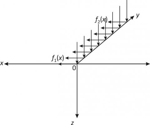
The two dimensional problem of elasticity involving half-space soil media considered in this study is shown in Figure 1, which illustrates general load f1(x) and f2(x) acting in the positive x and z coordinate directions on soil medium lying in the half plane $-\infty \leq x \leq \infty, 0 \leq z \leq \infty$
Figure 1. Loads f1(x) and f2(x) acting on half space soil.
The governing equations of plane strain elasticity are the differential equations of equilibrium, the stress compatibility equations and the stress-strain laws subject to the boundary conditions. The stress fields and strain fields in the half space are required to simultaneously satisfy all the governing equations.
The differential equations of equilibrium for an elemental part of the soil medium at any arbitrary point (x, y, z) in the semi-infinite mass on the xz plane are given by:
$\frac{\partial \sigma_{x x}}{\partial x}+\frac{\partial \tau_{x z}}{\partial z}+b_{x}=0$ (1)
$\frac{\partial \tau_{x z}}{\partial x}+\frac{\partial \sigma_{z z}}{\partial z}+b_{z}=0$ (2)
When bx = 0, bz = 0, the differential equations of equilibrium are simplified to be:
$\frac{\partial \sigma_{x x}}{\partial x}+\frac{\partial \tau_{x z}}{\partial z}=0$ (3)
$\frac{\partial \tau_{x z}}{\partial x}+\frac{\partial \sigma_{z z}}{\partial z}=0$ (4)
where bx and bz are the two body forces per unit volume, $\sigma_{x x}$ and $\sigma_{z z}$ are the normal stresses, and $\tau_{x z}$ is the shear stress; and x and z are the two dimensional Cartesian coordinates of the problem.
The compatibility equation in terms of stresses is:
$\frac{\partial^{2} \sigma_{x x}}{\partial z^{2}}+\frac{\partial^{2} \sigma_{z z}}{\partial x^{2}}=2 \frac{\partial^{2} \tau_{x z}}{\partial x \partial z}$ (5)
The stress-strain laws for linear elastic homogeneous, isotropic soil for plane strain conditions are given by the three relations:
$\varepsilon_{x x}=\frac{1}{E}\left[\left(1-\mu^{2}\right) \sigma_{x x}-\mu(1+\mu) \sigma_{z z}\right]$ (6)
$\varepsilon_{z z}=\frac{1}{E}\left[\left(1-\mu^{2}\right) \sigma_{z z}-\mu(1+\mu) \sigma_{x x}\right]$ (7)
$\gamma_{x z}=\frac{\tau_{x z}}{G}=\frac{2(1+\mu)}{E} \tau_{x z}$ (8)
where $\mu$ is the Poisson’s ratio, E is the Young’s modulus of elasticity and G is the shear modulus.
The boundary conditions are given by:
$\sigma_{x x} \cos (n, x)+\tau_{x z} \cos (n, z)=f_{1}(x)$ (9)
$\tau_{x z} \cos (n, x)+\sigma_{z z} \cos (n, z)=f_{2}(x)$ (10)
where cos (n, x) and cos (n, z) are the direction cosines.
On the xy coordinate plane, z = 0 and
$\tau_{x z}=f_{1}(x)=\tau_{x z}(z=0)$ (11)
$\sigma_{z z}=f_{2}(x)=\sigma_{z z}(z=0)$ (12)
Application of the exponential transform method
Since, $-\infty \leq x \leq \infty$ we apply the exponential Fourier transformation with respect to x to the governing differential equations of equilibrium and the compatibility equations to obtain:
$\int_{-\infty}^{\infty}\left(\frac{\partial \sigma_{x x}}{\partial x}+\frac{\partial \tau_{x z}}{\partial z}\right) e^{i \lambda x} d x=0$ (13)
$\int_{-\infty}^{\infty}\left(\frac{\partial \tau_{x z}}{\partial x}+\frac{\partial \sigma_{z z}}{\partial z}\right) e^{i \lambda x} d x=0$ (14)
$\int_{-\infty}^{\infty}\left(\frac{\partial^{2} \sigma_{x x}}{\partial z^{2}}+\frac{\partial^{2} \sigma_{z z}}{\partial x^{2}}-\frac{2 \partial^{2} \tau_{x z}}{\partial x \partial z}\right) e^{i \lambda x} d x=0$ (15)
where $\lambda$ is the exponential Fourier transform parameter.
From Equation (13)
$\int_{-\infty}^{\infty} \frac{\partial \sigma_{x x}}{\partial x} e^{i \lambda x} d x+\int_{-\infty}^{\infty} \frac{\partial \tau_{x z}}{\partial z} e^{i \lambda x} d x=0$ (16)
Simplifying,
$-i \lambda \int_{-\infty}^{\infty} \sigma_{x x} e^{i \lambda x} d x+\frac{\partial}{\partial z} \int_{-\infty}^{\infty} \tau_{x z} e^{i \lambda x} d x=0$ (17)
Let $\int_{-\infty}^{\infty} \sigma_{x x} e^{i \lambda x} d x=\overline{\sigma}_{x x}(\lambda, z)$ (18)
where $\overline{\sigma}_{x x}(\lambda, z)$ is the exponential Fourier transform of $\sigma_{x x}(x, z)$
and $\int_{-\infty}^{\infty} \tau_{x z} e^{i \lambda x} d x=\overline{\tau}_{x z}(\lambda, z)$ (19)
$\overline{\tau}_{x z}(\lambda, z)$ is the exponential Fourier transform of $\tau_{x z}(x, z)$
Then,
$-i \lambda \overline{\sigma}_{x x}(\lambda, z)+\frac{\partial}{\partial z} \overline{\tau}_{x z}(\lambda, z)=0$ (20)
or $\frac{\partial}{\partial z} \overline{\tau}_{x z}(\lambda, z)=i \lambda \overline{\sigma}_{x x}(\lambda, z)$ (21)
Also, from Equation (14),
$\int_{-\infty}^{\infty} \frac{\partial \tau_{x z}}{\partial x} e^{i \lambda x} d x+\int_{-\infty}^{\infty} \frac{\partial \sigma_{z z}}{\partial z} e^{i \lambda x} d x=0$ (22)
$-i \lambda \int_{-\infty}^{\infty} \tau_{x z} e^{i \lambda x} d x+\frac{\partial}{\partial z} \int_{-\infty}^{\infty} \sigma_{z z} e^{i \lambda x} d x=0$ (23)
$-i \lambda \overline{\tau}_{x z}(\lambda, z)+\frac{\partial}{\partial z} \overline{\sigma}_{z z}(\lambda, z)=0$ (24)
where $\overline{\sigma}_{z z}(\lambda, z)$ is the exponential Fourier transform of $\sigma_{z z}(x, z)$ and is given by:
$\overline{\sigma}_{z z}(\lambda, z)=\int_{-\infty}^{\infty} \sigma_{z z} e^{i \lambda x} d x$ (25)
From Equation (15), we have:
$\int_{-\infty}^{\infty} \frac{\partial^{2} \sigma_{x x}}{\partial z^{2}} e^{i \lambda x} d x-2 \int_{-\infty}^{\infty} \frac{\partial^{2} \tau_{x z}}{\partial x \partial z} e^{i \lambda x} d x+\int_{-\infty}^{\infty} \frac{\partial^{2} \sigma_{z z}}{\partial x^{2}} e^{i \lambda x} d x=0$ (26)
Simplifying,
$\frac{\partial^{2}}{\partial z^{2}} \int_{-\infty}^{\infty} \sigma_{x x} e^{i \lambda x} d x-2(-i \lambda) \frac{\partial}{\partial z} \int_{-\infty}^{\infty} \tau_{x z} e^{i \lambda x} d x+(-i \lambda)^{2} \int_{-\infty}^{\infty} \sigma_{z z} e^{i \lambda x} d x=0$ (27)
Thus,
$\frac{\partial^{2}}{\partial z^{2}} \overline{\sigma}_{x x}(\lambda, z)+2 i \lambda \frac{\partial}{\partial z} \overline{\tau}_{x z}(\lambda, z)-\lambda^{2} \overline{\sigma}_{z z}(\lambda, z)=0$ (28)
A close look at Equation (28) reveals that $\lambda$ is the exponential Fourier transform parameter, and the only space coordinate variable in the Equation is z, hence the equation is an ordinary differential equation with respect to the space coordinate variable z. Thus, Equation (28) is expressed as the ordinary differential equation (ODE):
$\frac{d^{2}}{d z^{2}} \overline{\sigma}_{x x}(\lambda, z)+2 i \lambda \frac{d}{d z} \overline{\tau}_{x z}(\lambda, z)-\lambda^{2} \overline{\sigma}_{z z}(\lambda, z)=0$ (29)
Using the results from Equations (21) and (24), Equation (29) becomes:
$-\frac{1}{\lambda^{2}} \frac{d^{4}}{d z^{4}} \overline{\sigma}_{z z}(\lambda, z)+2 \frac{d^{2}}{d z^{2}} \overline{\sigma}_{z z}(\lambda, z)-\lambda^{2} \overline{\sigma}_{z z}(\lambda, z)=0$ (30)
Alternatively, we have the fourth order ODE in $\overline{\sigma}_{z z}(\lambda, z)$
$\frac{d^{4}}{d z^{4}} \overline{\sigma}_{z z}(\lambda, z)-2 \lambda^{2} \frac{d^{2}}{d z^{2}} \overline{\sigma}_{z z}(\lambda, z)+\lambda^{4} \overline{\sigma}_{z z}(\lambda, z)=0$ (31)
Applying the exponential Fourier transforms to the boundary conditions at z = 0,
$\int_{-\infty}^{\infty} \tau_{x z}(x, 0) e^{i \lambda x} d x=\int_{-\infty}^{\infty} f_{1}(x) e^{i \lambda x} d x$ (32)
$\int_{-\infty}^{\infty} \sigma_{z z}(x, 0) e^{i \lambda x} d x=\int_{-\infty}^{\infty} f_{2}(x) e^{i \lambda x} d x$ (33)
From Equation (32), we have:
$\overline{\tau}_{x z}(\lambda, 0)=f_{1}(\lambda)$ (34)
From Equation (33), we have:
${{\bar{\sigma }}_{zz}}(\lambda ,0)={{f}_{2}}(\lambda )$ (35)
where ${{f}_{1}}(\lambda )$ is the exponential Fourier transform of f1(x) and ${{f}_{2}}(\lambda )$ is the exponential Fourier transform of f2(x).
Solutions for the stresses in the exponential Fourier transform space
The vertical stress field ${{\bar{\sigma }}_{zz}}(\lambda ,z)$ is found in the exponential Fourier transform space by solving the fourth order ODE Equation (31) subject to the boundary conditions. The other stresses ${{\bar{\sigma }}_{xx}}(\lambda ,z)$ and ${{\bar{\tau }}_{xz}}(\lambda ,z)$ are obtained from using Equations (24) and (21). We solve for ${{\bar{\sigma }}_{zz}}(\lambda ,z)$ in Equation (31) using the method of undermined parameters. The nature of the fourth order ODE suggests the assumption of a trial solution in the form:
${{\bar{\sigma }}_{zz}}(\lambda ,z)=\exp (mz)$ (36)
where m is an undetermined parameter.
Then for untrivial solutions, the characteristic polynomial becomes:
${{({{m}^{2}}-{{\lambda }^{2}})}^{2}}=0$ (37)
The roots are: $m=\pm \lambda $ twice(38)
The general solution becomes:
${{\bar{\sigma }}_{zz}}(\lambda ,z)=({{c}_{1}}+{{c}_{2}}z){{e}^{-|\lambda |z}}+({{c}_{3}}+{{c}_{4}}z){{e}^{|\lambda |z}}$ (39)
where c1, c2, c3 and c4 are the four constants of integration.
For bounded solutions, the stresses ${{\bar{\sigma }}_{zz}}$ are required to tend to zero as $z\to \infty ,$ Hence,
c3 = 0 (40)
c4 = 0 (41)
The bounded solutions for ${{\bar{\sigma }}_{zz}}(\lambda ,z)$ becomes:
${{\bar{\sigma }}_{zz}}(\lambda ,z)=({{c}_{1}}+{{c}_{2}}z){{e}^{-|\lambda |z}}$ (42)
The other stresses ${{\bar{\tau }}_{xz}}(\lambda ,z),$${{\bar{\sigma }}_{xx}}(\lambda ,z)$ are obtained from Equations (24) and (21).
Thus,
${{\bar{\tau }}_{xz}}(\lambda ,z)=\frac{1}{i\lambda }\frac{d}{dz}{{\bar{\sigma }}_{zz}}(\lambda ,z)$ (43)
${{\bar{\tau }}_{xz}}(\lambda ,z)=\frac{1}{i\lambda }\left( \frac{d}{dz}({{c}_{1}}+{{c}_{2}}z){{e}^{-|\lambda |z}} \right)$ (44)
${{\bar{\tau }}_{xz}}(\lambda ,z)=\frac{1}{i\lambda }\left\{ {{c}_{1}}\frac{d}{dz}{{e}^{-|\lambda |z}}+{{c}_{2}}\frac{d}{dz}(z{{e}^{-|\lambda |z}}) \right\}$ (45)
${{\bar{\tau }}_{xz}}(\lambda ,z)=i\left( ({{c}_{1}}+{{c}_{2}}z)-\frac{{{c}_{2}}}{\lambda } \right){{e}^{-|\lambda |z}}$ (46)
Also,
${{\bar{\sigma }}_{xx}}(\lambda ,z)=\frac{1}{i\lambda }\frac{d}{dz}{{\bar{\tau }}_{xz}}(\lambda ,z)$. (47)
${{\bar{\sigma }}_{xx}}(\lambda ,z)=\frac{1}{i\lambda }\left\{ \frac{d}{dz}i({{c}_{1}}+{{c}_{2}}z)-\frac{{{c}_{2}}}{\lambda } \right\}{{e}^{-|\lambda |z}}$ (48)
${{\bar{\sigma }}_{xx}}(\lambda ,z)=\left( \frac{2{{c}_{2}}}{\lambda }-({{c}_{1}}+{{c}_{2}}z) \right){{e}^{-|\lambda |z}}$ (49)
Using the boundary conditions, Equations (34) and (35), we obtain:
${{\bar{\tau }}_{xz}}(\lambda ,0)={{f}_{1}}(\lambda )=i\left( {{c}_{1}}-\frac{{{c}_{2}}}{\lambda } \right){{e}^{0}}=i\left( {{c}_{1}}-\frac{{{c}_{2}}}{\lambda } \right)$ (50)
${{\bar{\sigma }}_{zz}}(\lambda ,0)={{c}_{1}}(\lambda )={{f}_{2}}(\lambda )$ (51)
$\therefore i\left( {{c}_{1}}-\frac{{{c}_{2}}}{\lambda } \right)={{f}_{1}}(\lambda )$ (52)
${{f}_{2}}(\lambda )-\frac{{{c}_{2}}}{\lambda }=\frac{{{f}_{1}}(\lambda )}{i}=-i{{f}_{1}}(\lambda )$ (53)
$\frac{{{c}_{2}}}{\lambda }={{f}_{2}}(\lambda )+i{{f}_{1}}(\lambda )$ (54)
${{c}_{2}}=\lambda ({{f}_{2}}(\lambda )+i{{f}_{1}}(\lambda ))$ (55)
Hence,
${{\bar{\sigma }}_{zz}}(\lambda ,z)=\left( {{f}_{2}}(\lambda )+\lambda z({{f}_{2}}(\lambda )+i{{f}_{1}}(\lambda )) \right){{e}^{-|\lambda |z}}$] (56)
${{\bar{\tau }}_{xz}}(\lambda ,z)=i\left( {{f}_{2}}(\lambda )+\lambda z({{f}_{2}}(\lambda )+i{{f}_{1}}(\lambda ))-{{f}_{2}}(\lambda )+i{{f}_{1}}(\lambda ) \right){{e}^{-|\lambda |z}}$ (57)
${{\bar{\tau }}_{xz}}(\lambda ,z)=i\left( {{f}_{2}}(\lambda )+(\lambda z-1)({{f}_{2}}(\lambda )+i{{f}_{1}}(\lambda )) \right){{e}^{-|\lambda |z}}$ (58)
${{\bar{\sigma }}_{xx}}=\left( 2({{f}_{2}}(\lambda )+i{{f}_{1}}(\lambda ))-({{f}_{2}}(\lambda )+\lambda z({{f}_{2}}(\lambda )+i{{f}_{1}}(\lambda )) \right){{e}^{-|\lambda |z}}$ (59)
${{\bar{\sigma }}_{xx}}(\lambda ,z)=\left( -{{f}_{2}}(\lambda )+(2-\lambda z)({{f}_{2}}(\lambda )+i{{f}_{1}}(\lambda )) \right){{e}^{-|\lambda |z}}$ (60)
Equations (56), (58) and (60) are the expressions for the solutions for the stresses in the exponential Fourier transform space; and are in terms of the transformed space variables $\lambda $ and z.
Solutions for stresses in the physical (problem) domain
The stresses ${{\sigma }_{xx}}(x,z),\,\,{{\sigma }_{zz}}(x,z),\,\,{{\tau }_{xz}}(x,z)$ in the problem (physical) domain are obtained by inversion of the exponential Fourier transforms of the corresponding stresses in Equation (56), (58) and (60). Thus,
${{\sigma }_{zz}}(x,z)=\frac{1}{2\pi }\int\limits_{-\infty }^{\infty }{{{e}^{-i\lambda x}}{{{\bar{\sigma }}}_{zz}}(\lambda ,z)d\lambda }$ (61)
${{\sigma }_{zz}}(x,z)=\frac{1}{2\pi }\int\limits_{-\infty }^{\infty }{\left[ {{f}_{2}}(\lambda )+\lambda z({{f}_{2}}(\lambda )+i{{f}_{1}}(\lambda )) \right]{{e}^{-|\lambda |z}}{{e}^{-i\lambda x}}d\lambda }$ (62)
where
${{f}_{2}}(\lambda )=\int\limits_{-\infty }^{\infty }{{{e}^{i\lambda t}}{{f}_{2}}(t)\,dt}$ (63)
${{f}_{1}}(\lambda )=\int\limits_{-\infty }^{\infty }{{{e}^{i\lambda t}}{{f}_{1}}(t)\,dt}$ (64)
and t is an integration variable introduced to avoid confusion in the implementation of the integration in the Equation (62).
Then,
$+\,\,\frac{1}{2\pi }\int\limits_{-\infty }^{\infty }{\lambda z\left( \int\limits_{-\infty }^{\infty }{{{e}^{i\lambda t}}{{f}_{2}}(t)dt+i\int\limits_{-\infty }^{\infty }{{{f}_{1}}(t){{e}^{i\lambda t}}dt}} \right){{e}^{-|\lambda |z}}{{e}^{-i\lambda x}}d\lambda }$ (65)
${{\sigma }_{zz}}=\frac{1}{2\pi }\left\{ \int\limits_{-\infty }^{\infty }{{{f}_{2}}(t)dt}\int\limits_{-\infty }^{\infty }{{{e}^{-|\lambda |z}}{{e}^{i\lambda t}}{{e}^{-i\lambda x}}d\lambda } \right\}+\frac{1}{2\pi }\left\{ \int\limits_{-\infty }^{\infty }{\lambda z\,{{f}_{2}}(t)dt}\int\limits_{-\infty }^{\infty }{{{e}^{-|\lambda |z}}{{e}^{i\lambda t}}{{e}^{-i\lambda x}}d\lambda } \right.$
$+\,\,\,i\int\limits_{-\infty }^{\infty }{\lambda z\,{{f}_{1}}(t)dt}\left. \int\limits_{-\infty }^{\infty }{{{e}^{-|\lambda |z}}{{e}^{i\lambda t}}{{e}^{-i\lambda x}}d\lambda } \right\}$ (66)
${{\sigma }_{zz}}=\frac{1}{2\pi }\left\{ \int\limits_{-\infty }^{\infty }{{{f}_{2}}(t)dt}\int\limits_{-\infty }^{\infty }{(1+\lambda z){{e}^{-|\lambda |z+i\lambda (t-x)}}}d\lambda \right\}$
$+\,\,\frac{iz}{2\pi }\left\{ \int\limits_{-\infty }^{\infty }{\,{{f}_{1}}(t)dt}\int\limits_{-\infty }^{\infty }{\lambda {{e}^{-|\lambda |z+i\lambda (t-x)}}d\lambda } \right\}$ (67)
We note that the integrals are given by:
$\int\limits_{-\infty }^{\infty }{\lambda \exp (-\left| \lambda \right|z+i\lambda (t-x)d\lambda )}$
$=\int\limits_{-\infty }^{0}{\lambda \exp (-\left| \lambda \right|z+i\lambda (t-x))d\lambda }$
$+\int\limits_{0}^{\infty }{\lambda \exp (-\left| \lambda \right|z+i\lambda (t-x))d\lambda }$ (68)
$=\frac{4i(x-t)z}{{{({{z}^{2}}+{{(t-x)}^{2}})}^{2}}}$ (69)
Similarly,
$\int\limits_{-\infty }^{\infty }{(1+\lambda z)\exp (-\left| \lambda \right|z+i\lambda (t-x))d\lambda }=\frac{4{{z}^{3}}}{{{({{(x-t)}^{2}}+{{z}^{2}})}^{2}}}$ (70)
Hence,
${{\sigma }_{zz}}(x,z)=\frac{2{{z}^{2}}}{\pi }\int\limits_{-\infty }^{\infty }{\left\{ \frac{(x-t){{f}_{2}}(t)+z{{f}_{1}}(t)}{{{({{(x-t)}^{2}}+{{z}^{2}})}^{2}}} \right\}dt}$ (71)
Similarly,
${{\tau }_{xz}}(x,z)\,=\int\limits_{-\infty }^{\infty }{i\left( {{f}_{2}}(\lambda )\,+\,(\lambda z-1)({{f}_{2}}(\lambda )\,+\,i{{f}_{1}}(\lambda )) \right){{e}^{-|\lambda |z}}{{e}^{-i\lambda x}}d\lambda }$ (72)
${{\tau }_{xz}}=\int\limits_{-\infty }^{\infty }{i\left( {{f}_{2}}(\lambda )+(\lambda z-1){{f}_{2}}(\lambda ) \right){{e}^{-|\lambda |z}}{{e}^{-i\lambda x}}d\lambda }$
$+\,\,\int\limits_{-\infty }^{\infty }{{{i}^{2}}(\lambda z-1){{f}_{1}}(\lambda ){{e}^{-|\lambda |z}}{{e}^{-i\lambda x}}d\lambda }$ (73)
${{\tau }_{xz}}(x,z)=\frac{2z}{\pi }\int\limits_{-\infty }^{\infty }{\left\{ \frac{(x-t){{f}_{2}}(t)+z\,{{f}_{1}}(t)}{{{({{(x-t)}^{2}}+{{z}^{2}})}^{2}}} \right\}(x-t)dt}$ (74)
Also,
${{\sigma }_{xx}}(x,z)=\int\limits_{-\infty }^{\infty }{\left( -{{f}_{2}}(\lambda )+(2-\lambda z)({{f}_{2}}(\lambda )+i\,{{f}_{1}}(\lambda )) \right){{e}^{-|\lambda |z}}{{e}^{-i\lambda x}}d\lambda }$ (75)
${{\sigma }_{xx}}=\int\limits_{-\infty }^{\infty }{\left( -{{f}_{2}}(\lambda )+(2-\lambda z){{f}_{2}}(\lambda ) \right){{e}^{-|\lambda |z}}{{e}^{-i\lambda x}}d\lambda }$
$+\,\,\int\limits_{-\infty }^{\infty }{(2-\lambda z)i\,{{f}_{1}}(\lambda ){{e}^{-|\lambda |z}}{{e}^{-i\lambda x}}d\lambda }$ (76)
${{\sigma }_{xx}}(x,z)=\frac{2}{\pi }\int\limits_{-\infty }^{\infty }{\left\{ \frac{(x-t){{f}_{2}}(t)+z\,{{f}_{1}}(t)}{{{({{(x-t)}^{2}}+{{z}^{2}})}^{2}}} \right\}{{(x-t)}^{2}}dt}$ (77)
Solution for stresses due to vertical point load and horizontal point load at the origin O.
Let f1(x) and f2(x) be point loads of magnitudes F1 and F2 acting at the origin O. Then,
${{f}_{1}}(x)={{F}_{1}}\delta (t)$ (78)
${{f}_{2}}(x)={{F}_{2}}\delta (t)$ (79)
where F1 and F2 are constants and $\delta (t)$ is the Dirac delta function.
Then the stresses are
${{\sigma }_{zz}}(x,z)=\frac{2{{z}^{2}}}{\pi }\int\limits_{-\infty }^{\infty }{\left\{ \frac{(x-t){{F}_{2}}\delta (t)+z\,{{F}_{1}}\delta (t)}{{{({{(x-t)}^{2}}+{{z}^{2}})}^{2}}} \right\}dt}$ (80)
${{\sigma }_{zz}}(x,z)=\frac{2{{z}^{2}}}{\pi }\int\limits_{-\infty }^{\infty }{\left\{ \frac{(x-t){{F}_{2}}+z\,{{F}_{1}}}{{{({{(x-t)}^{2}}+{{z}^{2}})}^{2}}} \right\}\delta t\,dt}$ (81)
${{\sigma }_{zz}}(x,z)=\frac{2{{z}^{2}}}{\pi }\left( \frac{(x{{F}_{2}}+z\,{{F}_{1}}}{{{({{x}^{2}}+{{z}^{2}})}^{2}}} \right)$ (82)
${{\tau }_{xz}}=\frac{2z}{\pi }\int\limits_{-\infty }^{\infty }{\left( \frac{(x-t){{F}_{2}}\delta (t)+z\,{{F}_{1}}\delta (t)}{{{({{(x-t)}^{2}}+{{z}^{2}})}^{2}}} \right)(x-t)dt}$ (83)
${{\tau }_{xz}}=\frac{2z}{\pi }\int\limits_{-\infty }^{\infty }{\left( \frac{(x-t){{F}_{2}}+z\,{{F}_{1}}}{{{({{(x-t)}^{2}}+{{z}^{2}})}^{2}}} \right)(x-t)\delta t\,dt}$ (84)
${{\tau }_{xz}}=\frac{2zx}{\pi }\left( \frac{x{{F}_{2}}+z\,{{F}_{1}}}{{{({{x}^{2}}+{{z}^{2}})}^{2}}} \right)$ (85)
${{\sigma }_{xx}}(x,z)=\frac{2}{\pi }\int\limits_{-\infty }^{\infty }{\left( \frac{(x-t){{F}_{2}}\delta (t)+z\,{{F}_{1}}\delta (t)}{{{({{(x-t)}^{2}}+{{z}^{2}})}^{2}}} \right){{(x-t)}^{2}}dt}$ (86)
${{\sigma }_{xx}}(x,z)=\frac{2}{\pi }\int\limits_{-\infty }^{\infty }{\left( \frac{(x-t){{F}_{2}}+z\,{{F}_{1}}}{{{({{(x-t)}^{2}}+{{z}^{2}})}^{2}}} \right){{(x-t)}^{2}}\delta t\,dt}$ ](87)
${{\sigma }_{xx}}(x,z)=\frac{2{{x}^{2}}}{\pi }\left( \frac{x{{F}_{2}}+z\,{{F}_{1}}}{{{({{x}^{2}}+{{z}^{2}})}^{2}}} \right)$ (88)
For ${{F}_{1}}=0,\,\,\,{{F}_{2}}\ne 0$
${{\sigma }_{xx}}=\frac{2{{x}^{3}}{{F}_{2}}}{\pi {{r}^{4}}}$ (89)
where r2 = x2 + z2
${{\tau }_{xz}}=\frac{2z{{x}^{2}}{{F}_{2}}}{\pi {{r}^{4}}}$ (90)
${{\sigma }_{zz}}=\frac{2{{z}^{2}}x{{F}_{2}}}{\pi {{r}^{4}}}$ (91)
For ${{F}_{2}}=0,\,\,\,{{F}_{1}}\ne 0,$
${{\sigma }_{xx}}=\frac{2{{x}^{2}}z{{F}_{1}}}{\pi {{r}^{4}}}$ (92)
${{\tau }_{xz}}=\frac{2{{z}^{2}}x{{F}_{1}}}{\pi {{r}^{4}}}$ (93)
${{\sigma }_{zz}}=\frac{2{{z}^{3}}{{F}_{1}}}{\pi {{r}^{4}}}$ (94)
Solutions for stress fields due to uniformly distributed line load on one side of the x-axis
We consider the specific problem where a uniformly distributed line load of intensity p0 acts on one side of the x axis; in this case, the positive x-axis $x\ge 0.$ Then, the load f2(x) is expressed as
${{f}_{2}}(x)={{p}_{0}}\,H(x)$ (95)
where H(x) is the Heaviside function given by
$H(x)=\left\{ \begin{matrix} 1 & x\ge 0 \\ 0 & x<0 \\\end{matrix} \right.$ (96)
Then,
f1(t) = 0 (97)
Then,
${{\sigma }_{zz}}=\frac{2{{p}_{0}}{{z}^{3}}}{\pi }\int\limits_{0}^{\infty }{\frac{dt}{{{({{(x-t)}^{2}}+{{z}^{2}})}^{2}}}}$ (98)
${{\tau }_{xz}}=\frac{2{{p}_{0}}{{z}^{2}}}{\pi }\int\limits_{0}^{\infty }{\frac{(x-t)dt}{{{({{(x-t)}^{2}}+{{z}^{2}})}^{2}}}}$ (99)
${{\sigma }_{xx}}=\frac{2{{p}_{0}}z}{\pi }\int\limits_{0}^{\infty }{\frac{{{(x-t)}^{2}}dt}{{{({{(x-t)}^{2}}+{{z}^{2}})}^{2}}}}$ (100)
Let
$\frac{z}{x-t}=\tan \theta $ (101)
Let
$z=r\sin \theta $ (102)
$x=r\cos \theta $ (103)
$x-t=z\cot \theta =\frac{z}{\tan \theta }$ (104)
Then,
${{\sigma }_{zz}}={{p}_{0}}\left( 1-\frac{\theta }{\pi }+\frac{\sin 2\theta }{2\pi } \right)$ (105)
${{\tau }_{xz}}=-{{p}_{0}}\frac{{{\sin }^{2}}\theta }{\pi }$ (106)
${{\sigma }_{xx}}={{p}_{0}}\left( 1-\frac{\theta }{\pi }-\frac{\sin 2\theta }{2\pi } \right)$ (107)
where
$\theta ={{\sin }^{-1}}\frac{z}{r}={{\cos }^{-1}}\frac{x}{r}$ (108)
In this study, the exponential Fourier transform method was used to solve the elastic half plane problem on the xz coordinate plane involving loads acting on the surface of the boundary where the elastic half plane is assumed to be made of soil media that is linear elastic, isotropic, homogeneous and semi-infinite in extent with $-\infty \le x\le \infty ,$ and $0\le z\le \infty .$ The governing (field) equations are the differential equations of equilibrium, the compatibility equation expressed in terms of stress, the kinematic relations and the boundary conditions. The exponential Fourier transformation was applied to the governing differential equations of equilibrium and the compatibility equations expressed in terms of stress, to obtain, after algebraic processes, the fourth order ordinary differential equation (ODE) – Equation (31) – expressed in terms of the vertical stress fields in the exponential Fourier transform space. The exponential Fourier transformation was similarly applied to the boundary conditions to obtain the boundary conditions expressed in the exponential Fourier transform space as Equations (34) and (35). The fourth order ODE for ${{\bar{\sigma }}_{zz}}(\lambda ,z),$ vertical stress in the exponential Fourier transform space, was solved using the method of undetermined parameters to obtain the general solution given as Equation (39). The requirements for boundedness of the stresses were used to obtain the bounded solutions for ${{\bar{\sigma }}_{zz}}(\lambda ,z)$ as Equation (42). The other stresses ${{\bar{\tau }}_{xz}}(\lambda ,z),$${{\bar{\sigma }}_{xx}}(\lambda ,z),$ in the exponential transform space were obtained from Equation (42) using Equations (21) and (24), as Equations (46) and (49), respectively. Enforcement of boundary conditions yielded the unknown constants of integration as Equations (51) and (55). Thus the stresses become completely determined as Equations (56), (58) and (60) in the exponential transform space variables. Inversion of the exponential transforms for the stresses gave the general expressions for stresses in the physical domain space variables as Equations (67), (74) and (77).
Particular problems of elastic half plane problems under vertical and horizontal point loads at the origin, O, were considered. The stress fields for elastic half plane problems under combined vertical and horizontal point loads applied at the origin were found as Equations (82), (85) and (88). The stress fields for elastic half plane problems under vertical point load applied at the origin were found as Equations (89-91). The stress fields for elastic half plane problems under horizontal point load applied at the origin were found as Equations (92-94). Similarly, the specific problem of an elastic half plane under uniformly distributed line load p0 applied to one side of the x-axis was considered and the stress fields were obtained as Equations (105-107). It was observed that the expressions obtained were identical with expressions obtained by other researchers who used other methods of solution.
The conclusions of this study are as follows:
(i) The exponential Fourier transform method has been successfully used in this paper to obtain general solutions for the stresses in a linear elastic, isotropic, homogeneous soil medium in the xz coordinate plane under boundary loads.
(ii) The exponential Fourier transform method has been successfully implemented in this paper to find solutions for stresses in elastic half plane media due to line loads of constant intensity acting along the x axis.
(iii) The exponential Fourier transform method has been successfully implemented in this work to find stresses due to vertical and horizontal point loads applied at the origin O of an elastic half plane medium (on the xz coordinate plane) considered linear elastic, isotropic and homogeneous.
[1] Vertical Stress in a Soil Mass. www.civil.uwaterloo.ca/maknight/courses/CiVE353/Lectures/stress-load.pdf
[2] Lecture Note Course Code BCE 402 Geotechnical Engineering II Stress Distribution in Soil-VSSUT https//www.vssut.ac/in/lecture_notes/lecture1424085471.pdf
[3] Fredlund DG, Rahardjo H, Fredlund MD. (2012). Unsaturated Soil Mechanics in Engineering Practice. https/books.google.com/books isbn=1118280504.
[4] Onah HN, Osadebe NN, Ike CC, Nwoji CU. (2016). Determination of stresses caused by infinitely long line loads on semi-infinite elastic soils using Fourier transform method. Nigerian Journal of Technology (NIJOTECH) 35(4): 726-731.
[5] Ike CC. (2006). Principles of Soil Mechanics. De-Adroit Innovation, Enugu.
[6] Timoshenko S. (1948). Theory of Elasticity. McGraw Hill Book Co., New York, 338-339.
[7] Das BM. (2008). Advanced Soil Mechanics. Third Edition. Taylor and Francis, London and New York.
[8] Verruijt A. (2006). Soil Mechanics. Delft University of Technology.
[9] Richards R. (2001). Principles of Solid Mechanics. CRC Press, Washington D.C.
[10] Cummings A.E. (1936). Distribution of stresses under a foundation Transactions, American Society of Civil Engineers 101: 1072-1134.
[11] Gray H. (1936). Stress distribution in elastic solids. Proceedings of International Conference on Soil Mechanics and Foundation Engineering Cambridge 2: pp. 157-168.
[12] Newmark NM. (1940). Stress distribution in soils. Proceedings Purdue Conference on Soil Mechanics and its Applications, pp. 295-303.
[13] Holl DL (1941). Plane strain distribution of stress in elastic media. Iowa Engineering Experiment Station, Bull 148: 55
[14] Forster CR, Fergus SM. (1951). Stress distribution in a homogeneous soil. Research Report No 12-F. Highway Research Board, p. 36.