Sheela Khatun | Md. Tusher Mollah | Mst. Sonia Akter | Muhammad Minarul Islam | Md. Mahmud Alam*
OPEN ACCESS
The Numerical study for the unsteady electro magneto-hydrodynamic (EMHD) Couette flow of Bingham fluid through a porous parallel Riga plates with the consideration of thermal radiation has been carried out. The Couette flow is considered where the upper Riga plate moves with a uniform velocity U0 and the lower Riga plate is stationary. An external uniform magnetic field is applied perpendicular to the plates. Both the upper and lower Riga plates are kept at different but constant temperatures T1 and T2. respectively, where T2>T1. The governing equations have been transformed into dimensionless non-linear partial differential equations by using usual transformations. The obtained equations have been solved numerically by the explicit finite difference method (FDM) under the stability and convergence analysis. The effects of some important parameters on shear stress, Nusselt number including velocity and temperature distributions have been discussed graphically by MATLAB R2015a.
MHD, Bingham fluid, Riga plate, finite difference method, stability analysis
The flow of non-Newtonian fluids in the presence of heat transfer is an important research area due to its wide use in food processing, power engineering and petroleum production and in many industries for example polymers melt and polymer solutions employed in the plastic processing. A special class of non-Newtonian viscoplastic fluid that exhibit a linear behavior of shear stress versus shear rate once the fluid begins to flow is known as Bingham fluid. It behaves as a rigid body at low stress but flows as a viscous fluid at high stress. A common example is toothpaste, which will not be extruded until a certain pressure is applied to the tube. The MHD Bingham fluid flow is used in many geological and industry materials as a common mathematical model of mud flow in drilling engineering, and in the handling of slurries, lava, cement etc. Bingham fluid is named after Eugene C. Bingham [1] who mentioned its mathematical form.
In this consequence, the physical and chemical properties of the Bingham fluid have been described by Bingham [2]. Darby and Melson [3] developed an experimental formulation to prophesy the friction factor for a flow of Bingham plastics. Vola et al. [4] also studied a numerical strategy and some benchmark results of laminar unsteady flows of Bingham fluids. The numerical simulation of Taylor Couette flow of Bingham fluids has been investigated by Jeng and Zhu [5]. Sreekala and Kesavareddy [6] investigated the Hall effects on unsteady MHD flow of a Non-Newtonian fluid through a Porous medium with uniform suction and injection. Parvin, et al. [7] studied the unsteady MHD viscous incompressible Couette flow of Bingham fluid with hall current. Tlili et al. [8] considered the first- and second-law analyses of MHD Couette–Poiseuille flow of water-based nanofluids in a rotating permeable channel by Buongiorno model and the impacts of Hall current, radiation, variable viscosity, thermophoresis, including Brownian motion. Mollah et al. [9] studied the Hall and Ion-slip effects on unsteady MHD Bingham fluid flow with suction.
Riga plate is the termed as an electromagnetic actuator which is formed by the combination of permanent magnets and a span wise aligned array of alternating electrodes mounted on a plane surface. It is numerously used for the radiation of an efficient agent, skin friction and pressure drag of submarines by avoiding the boundary layer separation. In this regard, the laminar fluid flow along Riga plate has been investigated in various physical aspects.
The Riga plate is considered by Gailitis and Lielausis [10] to build an applied magnetic and electric fields which consequently generates Lorentz force parallel to the wall due to control the flow of fluid. The EMHD free-convection boundary-layer flow from a Riga-plate has been investigated by Pantokratoras and Magyari [11]. Ahmad et al. [12] studied the flow of nanofluid past a Riga plate. The squeezing flow past a Riga plate with chemical reaction and convective conditions has been considered by Hayat et al. [13]. Iqbal, et al. [14] considered the numerical investigation of nanofluidic transport of gyrotactic microorganisms submerged in the water towards Riga plate. A numerical approach for the radiative Williamson nanofluid flow over a convectively heated Riga plate with chemical reaction has been investigated by Ramzan et al. [15]. Ramesh and Gireesha [16] studied the non-linear Radiative flow of nanofluid past a moving or stationary Riga plate. The analytical investigation of third grade nanofluidic flow over a Riga plate using Cattaneo-Christov model has been considered by Naseem et al. [17]. Anjum et al. [18] investigated the influence of thermal stratification and slip conditions on stagnation point flow towards variable thick Riga plate.
Along with the above studies, the present study focuses on unsteady EMHD Couette flow of Bingham fluid through a porous parallel Riga plates with the consideration of thermal radiation. The study concerned with the Lorentz force along the X-axis which is thereafter advances into an exponential function according to the Grinberg term. The pressure gradient, thermal radiation and porous medium are also considered. The explicit finite difference technique has been used to solve the dimensionless non-linear partial differential equations. The obtained results have been shown graphically.
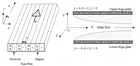
The viscous incompressible Bingham fluid is assumed to be flowing between two infinite horizontal non-conducting porous Riga plates which are placed at $y=\pm h\,$ planes and extend from $x=0\,\text{to}\,\,\infty \,$ and from $\,\text{z=0}\,\,\text{to}\,\,\infty $. The Couette flow is considered where, the lower Riga plate is taken to be stationary while the upper Riga plate is moving with uniform velocity ${{U}_{0}}$. Both the lower and upper plates are taken at two constant temperatures ${{T}_{1}}\,\,\text{and}\,\,{{T}_{2}}$respectively, where ${{T}_{2}}>{{T}_{1}}$. In the X-direction, a constant pressure gradient $\frac{dp}{dx}$is applied along the fluid flow. Here, the fluid velocity vector is given as follows:
$\mathbf{\tilde{q}}=\tilde{u}\mathbf{i}+\tilde{v}\mathbf{j}$.
For the Riga plate the volume density of a Lorentz force can be written in vector product form as $\mathbf{F=J}\wedge \mathbf{B}$ ; where, the current density by means of Ohm’s law can be written as follows:
$\mathbf{J}=\sigma \left( \mathbf{E+\tilde{q}}\wedge \mathbf{B} \right)$
Since the Bingham fluid is weakly conducting ($\sigma ={{10}^{6}}\text{S/m}$or very small) then the current density $\sigma \left( \mathbf{\tilde{q}}\wedge \mathbf{B} \right)$is small. So that the term $\sigma \left( \mathbf{\tilde{q}}\wedge \mathbf{B} \right)$ in the above equation, can be neglected. Thus, to obtain the EMHD flow, the extrinsic magnetic field is used which is the Lorentz force along the X-axis and can be written as follows:
$\mathbf{F}=\mathbf{J}\wedge \mathbf{B}\approx \sigma \left( \mathbf{E}\wedge \mathbf{B} \right)$
According to the Grinberg term$\left( \frac{\mathbf{F}}{\rho } \right)$, the density force$\mathbf{F}=\mathbf{Fex}$, averaged over a span wise coordinate along Z-axis, which advances into an exponential function of y, can be expressed as follows:
$F=\frac{\pi }{8}{{J}_{0}}{{M}_{0}}\exp \left( -\frac{\pi }{a}y \right)$ where, ${{J}_{0}}\,\left( A/{{m}^{2}} \right)$
where, $J_{0}\left(A / m^{2}\right)$ is the applied current density in the electrodes, $M_{0}(\text { Tesla })$ is the magnetization of the permanent magnets and $a$ is the width of magnets and electrodes.
The Rosse land approximation for thermal radiation can be written as follows:
${{Q}_{r}}=-\frac{4{{\sigma }^{*}}}{3{{k}^{*}}}\left( \frac{\partial {{T}^{4}}}{\partial y} \right)$
where, mean absorption coefficient (${{k}^{*}}$), radiative heat flux (${{Q}_{r}}$) and Stefan-Boltzmann constant (${{\sigma }^{*}}$). The Taylor series for ${{T}^{4}}$about ${{T}_{\infty }}$ implies ${{T}^{4}}\cong 4T_{\infty }^{3}-3T_{\infty }^{4}$, which gives the following form for thermal radiation:
${{Q}_{r}}=-\frac{16{{\sigma }^{*}}}{3{{k}^{*}}}T_{\infty }^{3}\frac{\partial T}{\partial y}$
Figure 1. Schematic physical configuration of the problem
Within the framework of the above assumptions, the unsteady model for the EMHD Couette flow of Bingham fluid through a porous parallel Riga plates with the consideration of thermal radiation is governed by the continuity, momentum and energy equations under the boundary-layer approximations, which can be written as follows:
$\frac{\partial \tilde{u}}{\partial x}+\frac{\partial \tilde{v}}{\partial y}=0$ (1)
$\frac{\partial \tilde{u}}{\partial t}+\tilde{u}\frac{\partial \tilde{u}}{\partial x}+\tilde{v}\frac{\partial \tilde{u}}{\partial y}=-\frac{1}{\rho }\frac{dp}{dx}+\frac{1}{\rho }\frac{\partial }{\partial y}\left( \tilde{\mu }\frac{\partial \tilde{u}}{\partial y} \right)+\frac{\pi }{8\rho }{{J}_{0}}{{M}_{0}}\exp \left( -\frac{\pi }{a}y \right)-\frac{\upsilon }{k'}\tilde{u}$ (2)
$\frac{\partial \tilde{T}}{\partial t}+\tilde{u}\frac{\partial \tilde{T}}{\partial x}+\tilde{v}\frac{\partial \tilde{T}}{\partial y}=\frac{\kappa }{{{c}_{p}}\rho }\left( \frac{{{\partial }^{2}}\tilde{T}}{\partial {{y}^{2}}} \right)+\frac{{\tilde{\mu }}}{\rho {{c}_{p}}}{{\left( \frac{\partial \tilde{u}}{\partial y} \right)}^{2}}+\frac{1}{\rho {{c}_{p}}}\frac{16{{\sigma }^{*}}}{3{{k}^{*}}}T_{2}^{3}\frac{{{\partial }^{2}}\tilde{T}}{\partial {{y}^{2}}}$ (3)
where, $\tilde{\mu }=K+\frac{{{\tau }_{0}}}{\left( \frac{\partial \tilde{u}}{\partial y} \right)}$ (4)
and the corresponding initial and boundary conditions for the problem are:
$t\le 0,\,\,\,\text{ }\,\,\tilde{u}=0,\,\,\,\text{ }\tilde{T}={{T}_{1}}$ everywhere (5)
$\begin{align} & \,\,\,\,\,\,\,\,\,\,\,\,\,\,\,\,\,\,\,\,\,\,\,\tilde{u}=0,\,\,\,\,\,\,\,\,\,\tilde{T}={{T}_{1}}\,\,\,\,\,\,\,\,\,\text{at}\,\,x\text{=0} \\ & t>0,\,\,\,\,\,\,\,\,\,\text{ }\tilde{u}=0,\,\,\,\,\,\,\,\,\,\tilde{T}={{T}_{1}}\,\,\,\,\,\,\,\,\,\text{at}\,\,y=-h \\ & \,\,\,\,\,\,\,\,\,\,\,\,\,\,\,\,\,\,\,\,\,\,\tilde{u}={{U}_{0}},\,\,\text{ }\tilde{T}={{T}_{2}}\,\,\,\,\,\,\,\,\text{at}\,\,\,y=h \\ \end{align}$ (6)
It is required to transform the equations (1) to (4) into dimensionless form, as the solution of these equations with the initial conditions and boundary conditions (5) and (6) will be based on the FDM for numerical solution. The dimensionless quantities that have used are given as follows:
$\begin{align} & X=\frac{x}{h},Y=\frac{y}{L},U=\frac{{\tilde{u}}}{{{U}_{0}}},V=\frac{{\tilde{v}}}{{{V}_{0}}},P=\frac{p}{\rho U_{0}^{2}},\tau =\frac{t{{U}_{0}}}{h},\bar{\mu }=\frac{{\tilde{\mu }}}{K}\text{and }\theta =\frac{\tilde{T}-{{T}_{1}}}{{{T}_{2}}-{{T}_{1}}}, \\ & \text{where,}\,\,{{V}_{0}}=\frac{\upsilon \pi }{a},h=\frac{{{U}_{0}}{{L}^{2}}}{\upsilon },L=\frac{a}{\pi } \\ \end{align}$ (7)
The obtained dimensionless differential equations are presented as follows:
$\frac{\partial U}{\partial X}+\frac{\partial V}{\partial Y}=0$ (8)
$\frac{\partial U}{\partial \tau }+U\frac{\partial U}{\partial X}+V\frac{\partial U}{\partial Y}=-\frac{dP}{dX}+\frac{1}{{{R}_{e}}}\frac{\partial }{\partial Y}\left( \bar{\mu }\frac{\partial U}{\partial Y} \right)+Z{{e}^{-Y}}-{{k}_{0}}U$ (9)
$\frac{\partial \theta }{\partial \tau }+U\frac{\partial \theta }{\partial X}+V\frac{\partial \theta }{\partial Y}=\left( \frac{1}{{{P}_{r}}}+\frac{4}{\text{3}}{{R}_{D}} \right)\frac{{{\partial }^{2}}\theta }{\partial {{Y}^{2}}}+{{E}_{c}}\bar{\mu }{{\left( \frac{\partial U}{\partial Y} \right)}^{2}}$ (10)
$\bar{\mu }=1+\frac{{{\tau }_{D}}}{\left( \frac{\partial U}{\partial Y} \right)}$ (11)
and the dimensionless conditions are mentioned as follows:
$\tau \le 0,\,\text{ }\,\,\,\,U=0,\text{ }\theta =0$ everywhere (12)
$\begin{align} & \,\,\,\,\,\,\,\,\,\,\,\,\,\,\,\,\text{ }\,U=0,\text{ }\theta =0\,\,\,\text{ }\,\text{at}\,\,X\text{=0} \\ & \tau >0,\text{ }\,\,\,U=0,\text{ }\theta =0\,\,\,\,\text{ at}\,\,Y=-1 \\ & \,\,\,\,\,\,\,\,\,\,\,\,\,\,\,\text{ }\,U=1,\text{ }\theta =1\,\,\,\text{ }\,\text{at}\,\,\,Y=1 \\ \end{align}$ (13)
The non-dimensional parameters are given as follows:
${{R}_{e}}=\frac{\rho {{V}_{0}}L}{K}$(Reynolds number); ${{P}_{r}}=\frac{\rho {{c}_{p}}{{U}_{0}}{{L}^{2}}}{kh}$ (Prandtl number); $Z=\frac{{{J}_{0}}{{M}_{0}}{{a}^{2}}}{8\pi \rho {{U}_{0}}\upsilon }$ (Modified Hartmann number); ${{E}_{C}}=\frac{{{U}_{0}}Kh}{\rho {{c}_{p}}{{L}^{2}}({{T}_{2}}-{{T}_{1}})}$ (Eckert number); ${{R}_{D}}=\frac{4{{\sigma }^{*}}T_{2}^{\text{3}}}{k{{\kappa }^{*}}}$ (Radiation parameter), Permeability of porous medium, ${{k}_{0}}=\frac{{{\upsilon }^{2}}}{k{{U}_{0}}^{2}}$ and ${{\tau }_{D}}=\frac{{{\tau }_{0}}h}{K{{U}_{0}}}$ (Bingham number or dimensionless yield stress).
The effects of various parameters on shear stress have been studied from the velocity profile. The local shear stress in X- direction for upper (moving) wall is ${{\tau }_{L}}\equiv \mu {{\left( \frac{\partial U}{\partial Y} \right)}_{Y=1}}$.
Also, the effects of various parameters on Nusselt number have been studied from the temperature profile. The local Nusselt number in X- direction for upper (moving) wall is $N{{u}_{L}}\equiv \frac{{{\left( \frac{\partial T}{\partial Y} \right)}_{Y=1}}}{-\left( {{T}_{m}}-1 \right)}$, where ${{T}_{m}}$is the dimensionless mean fluid temperature and is given by ${{T}_{m}}=\frac{\int\limits_{-1}^{1}{U\theta dY}}{\int\limits_{-1}^{1}{UdY}}$.
A set of finite difference approach is required to solve the dimensionless non-linear partial differential equations (8) to (11) by the explicit FDM subjected to boundary conditions. Therefore, the region interior to the boundary layer is distributed into a grid of lines perpendicular to Y-axis.
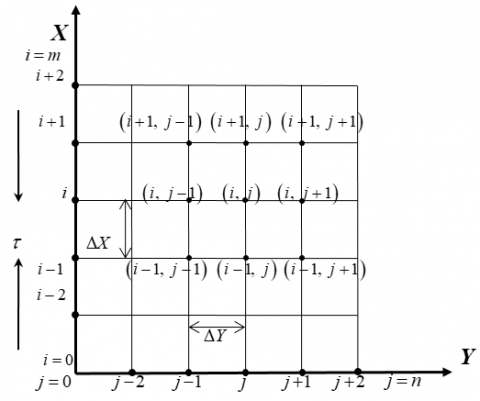
Here it is considered that the height of the plate ${{X}_{\max }}\left( =40 \right)$ i.e. X changes from 0 to 40 and regard ${{Y}_{\max }}\left( =2 \right)$ as corresponding to $Y\to \infty $ i.e. Y changes from 0 to 2. Also $m=40$ and $n=40$ mesh spacing are considered in the X and Y directions respectively as shown in Fig. 2.
It is assumed that $\Delta X$, $\Delta Y$ are constant mesh sizes along X and Y directions respectively and taken as follows:
$\Delta X=1.0\,\left( 0\le x\le 40 \right)$, $\Delta Y=0.05\,\left( 0\le y\le 2 \right)$ with the smaller time-step, $\Delta \tau =0.0001$.
Figure 2. Finite difference space grid
Let $U'$ and $\theta '$ represents the magnitudes of $U$ and $\theta $ at the final time-step respectively. With the help of the explicit FDM approach the suitable set of finite difference equations are obtained as follows:
$\frac{{{U}_{i,\,j}}-{{U}_{i-1,\,j}}}{\Delta X}+\frac{{{V}_{i,\,j}}-{{V}_{i,\,j-1}}}{\Delta Y}\,=0$ (14)
$\begin{align} & \frac{{{{{U}'}}_{i,\,j}}-{{U}_{i,\,j}}}{\Delta \tau }+{{U}_{i,j}}\frac{{{U}_{i,\,j}}-{{U}_{i-1,\,j}}}{\Delta X}+{{V}_{i,j}}\frac{{{U}_{i,\,j}}-{{U}_{i,\,j-1}}}{\Delta Y}=-\frac{dP}{dX}+Z{{e}^{-Y}}-{{k}_{0}}{{U}_{i,j}} \\ & \,\,\,\,\,\,\,\,\,\,\,\,\,\,\,\,\,\,\,\,\,\,\,\,\,\,\,\,\,\,\,\,\,+\frac{1}{{{R}_{e}}}\left[ \left( \frac{{{{\bar{\mu }}}_{i,\,j}}-{{{\bar{\mu }}}_{i,\,j-1}}}{\Delta Y} \right)\left( \frac{{{U}_{i,\,j}}-{{U}_{i,\,j-1}}}{\Delta Y} \right)+{{{\bar{\mu }}}_{i,\,j}}\left( \frac{{{U}_{i,\,j+1}}-2{{U}_{i,\,j}}+{{U}_{i,\,j-1}}}{{{\left( \Delta Y \right)}^{2}}} \right) \right] \\ \end{align}$ (15)
$\begin{align} & \frac{\theta {{'}_{i,\,j}}-{{\theta }_{i,\,j}}}{\Delta \tau }+{{U}_{i,j}}\frac{{{\theta }_{i,\,j}}-{{\theta }_{i-1,\,j}}}{\Delta X}+{{V}_{i,j}}\frac{{{\theta }_{i,\,j}}-{{\theta }_{i,\,j-1}}}{\Delta Y}=\left( \frac{1}{{{P}_{r}}}+\frac{4}{\text{3}}{{R}_{D}} \right)\frac{{{\theta }_{i,\,j+1}}-2{{\theta }_{i,\,j}}+{{\theta }_{i,\,j-1}}}{{{\left( \Delta Y \right)}^{2}}} \\ & \,\,\,\,\,\,\,\,\,\,\,\,\,\,\,\,\,\,\,\,\,\,\,\,\,\,\,\,\,\,\,\,\,\,\,\,\,\,\,\,\,\,\,\,\,\,\,\,\,\,\,\,\,\,\,\,\,\,\,\,\,\,\,\,\,\,\,\,\,\,\,\,\,\,\,\,\,\,\,\,\,\,\,\,\,\,\,\,\,\,\,\,\,\,\,\,\,\,\,\,\,\,\,\,\,\,\,\,\,\,\,\,\,\,\,\,\,\,\,\,+{{E}_{c}}\left( {{{\bar{\mu }}}_{i,\,j}} \right){{\left( \frac{{{U}_{i,\,j}}-{{U}_{i,\,j-1}}}{\Delta Y} \right)}^{2}} \\ \end{align}$ (16)
${{\bar{\mu }}_{i,\,j}}=1+\frac{{{\tau }_{D}}}{\left( \frac{{{U}_{i,\,j}}-{{U}_{i,\,j-1}}}{\Delta Y} \right)}$ (17)
and the boundary conditions with FDM are:
$\begin{align} & {{U}_{i,L}}=0,\,\,{{W}_{i,L}}=0,\,\,{{\theta }_{i,L}}=0\,\,\,\text{at}\,\,L=-1 \\ & {{U}_{i,L}}=0,\,\,{{W}_{i,L}}=0,\,\,{{\theta }_{i,L}}=1\,\,\,\text{at}\,\,L=1 \\ \end{align}$.
Excluding the stability and convergence criteria of the finite difference method, the analysis will remain incomplete since an explicit procedure is being used. For the considered problem the stability and convergence criteria finally can be expressed as follows:
$\frac{U\Delta \tau }{\Delta X}-\frac{\left| V \right|\Delta \tau }{\Delta Y}+\left( \frac{1}{{{P}_{r}}}+\frac{4{{R}_{D}}}{3} \right)\frac{2\Delta \tau }{{{\left( \Delta Y \right)}^{2}}}+\frac{\Delta \tau }{2{{k}_{0}}}\le 1$
Using $\Delta Y=0.05,\,\,\Delta \tau =0.0001$ and the initial condition, the above equations gives ${{P}_{r}}\ge 0.09\text{ }$ when$\,{{R}_{D}}\le 1.00$and $\,{{k}_{0}}\le 5.00$.
Due to investigate the physical situation of the developed mathematical model, the steady-state numerical values have been computed for the non-dimensional velocity $\left(U \right)$ and temperature $\left( \theta \right)$within the boundary layer. Firstly, the mesh sensitivity has been discussed to obtain the appropriate grid spacing for the numerical calculation. Secondly, the time sensitivity has been explained to obtain the steady-state solution. Thirdly, the effect of Reynolds number $\left( {{R}_{e}} \right)$ and modified Hartmann number $\left( Z \right)$ on the velocity $\left( U \right)$ and temperature $\left( \theta \right)$ distributions as well as on the local shear stress at the upper plate $\left( {{\tau }_{L}} \right)$and local Nusselt number at the upper plate $\left( N{{u}_{L}} \right)$ are discussed graphically. Furthermore, for brevity, the effect of other parameters such as Prandtl number $\left( {{P}_{r}} \right)$, Eckert number $\left( {{E}_{c}} \right)$, Radiation parameter $\left( {{R}_{D}} \right)$, Permeability of porous medium $\left( {{k}_{0}} \right)$ and Bingham number $\left( {{\tau }_{D}} \right)$ are shown in tabular form. At last, the present result has been compared with several published results.
6.1 Examine mesh sensitivity
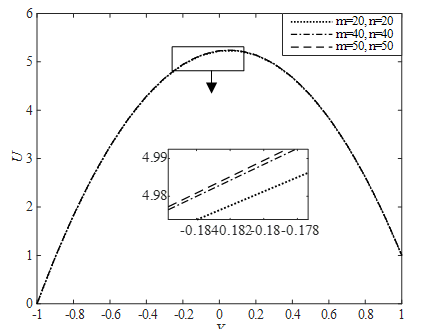
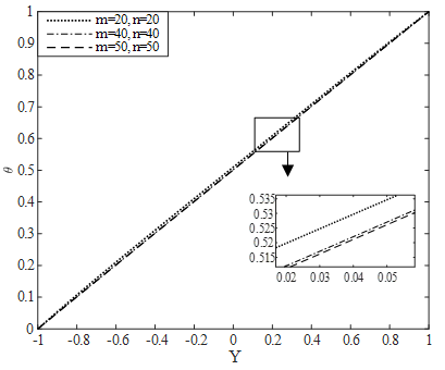
To find out the appropriate mesh for $m$ and $n$, the computations have been carried out for three different mesh such as $m\text{=20,}\,\text{ }n=20\,;\,\,$ $m\text{=40,}\,\text{ }n\text{=40}$ and $m=50,\,\text{ }n=50$ as shown in Figs. 3 and 4; where, ${{R}_{e}}=\,2.00,$ $Z=1.50,$ ${{R}_{D}}=\,0.05,$ ${{E}_{c}}=0.10,$ ${{P}_{r}}=\,1.50,$ ${{k}_{0}}=\,0.10$ and${{\tau }_{D}}=\,0.001$. The obtained curves are smooth for all mesh and shows a negligible change among these curves. For $m\text{=40,}\,\text{ }n\text{=40}$ and $m=50,\,\text{ }n=50$, the curves are quite same. Thus, $m\text{=40}\,\,\text{and}\,\,n\text{=40}$can be chosen as the appropriate mesh size.
Figure 3. Illustration of mesh sensitivity for Velocity Profiles
Figure 4. Illustration of mesh sensitivity for Temperature Profiles
6.2 Time sensitivity test
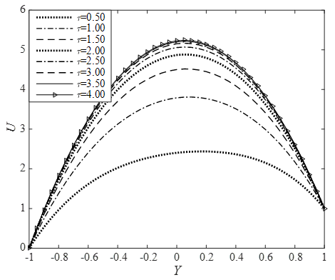
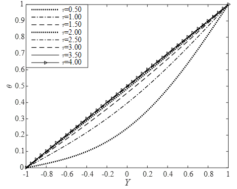
To complete the time sensitivity test of the developed mathematical model, the computations for $U$ and $\theta $ have been continued for different dimensionless time step sizes such as $\tau =$0.50, 1.00, 1.50, 2.00, 2.50, 3.00, 3.50 and 4.00 where, ${{R}_{e}}=\,2.00,$ $Z=1.50,$ ${{R}_{D}}=\,0.05,$ ${{E}_{c}}=0.10,$ ${{P}_{r}}=\,1.50,$ ${{k}_{0}}=\,0.10$ and${{\tau }_{D}}=\,0.001$. It is observed that, the result of computations for different profiles, however shows little changes after $\tau =$2.50 and shows negligible changes up to $\tau =$4.00. Thus the solutions of all variables for $\tau =$4.00 are taken essentially as the steady-state solutions. The time sensitivity for $U$ and $\theta $are shown in Figs. 5 and 6.
Figure 5. Illustration of time sensitivity for Velocity Profiles
Figure 6. Illustration of time sensitivity for Temperature Profiles
It is seen from Figures. 5 and 6 that both velocity and temperature profiles reach their steady state monotonically. It also should be mentioned that the temperature profile reaches the steady state faster than the velocity profile.
6.3 Effect of parameters
In order to achieved the clear concept of physical properties of the developed model, the effects of two parameters such as ${{R}_{e}}$ and $Z$, in the presence of ${{R}_{D}}=\,0.05,$ ${{E}_{c}}=0.10,$ ${{P}_{r}}=\,1.50,$ ${{k}_{0}}=\,0.10$ and ${{\tau }_{D}}=\,0.001$ at the steady-state dimensionless time$\tau =\,4.00$ are presented graphically through Figs. 7-14. For brevity, the effect of the other parameters are shown in tabular form (Table 1).
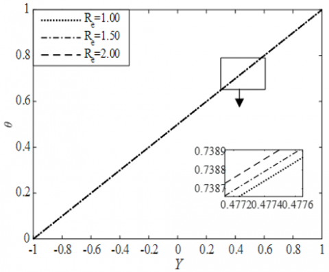
The effects of Reynolds number $\left( {{R}_{e}} \right)$ on $U$ and $\theta $ distributions as well as ${{\tau }_{L}}$ and $N{{u}_{L}}$ are presented in Figures. 7-10. Here, curves are plotted for the three different values of ${{R}_{e}}$ such as 1.00, 1.50 and 2.00 at the steady-state dimensionless time$\tau =\,4.00$. From Figures. 7 and 8 it is observed that, both the velocity and temperature distributions increase with the increase of ${{R}_{e}}$. It is seen from Figs. 9 and 10 that, both the local shear stress and local Nusselt number at upper plate decrease with the rise of ${{R}_{e}}$.
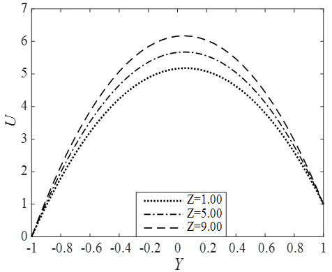
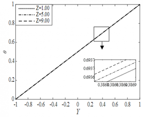
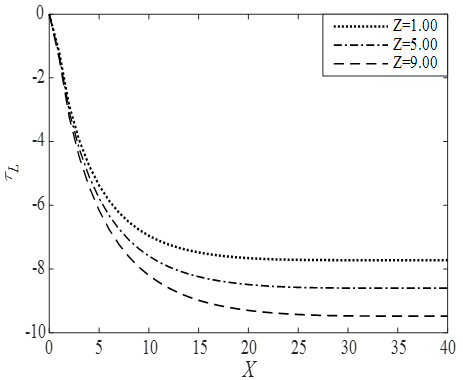
Furthermore, the effects of modified Hartmann number $\left( Z \right)$ on $U$ and $\theta $ distributions as well as ${{\tau }_{L}}$ and $N{{u}_{L}}$ are presented in Figs. 11-14. Here, curves are plotted for the three different values of $Z$ such as 1.00, 5.00 and 9.00 at the steady-state dimensionless time$\tau =\,4.00$. From Figures. 11 and 12, it is cleared that, both the velocity and temperature distributions increase with the increment of $Z$. It is seen from Figures. 13 and 14 that, both the local shear stress and local Nusselt number at upper plate decrease with the increment of $Z$.
Figures 7 and 8 show that, both the velocity and temperature distributions increase with the increase of Re.
Figures 9 and 10 show that, both the local shear stress and local Nusselt number at upper plate decrease with the increment of Re.
Figure 7. Effects of Re on Velocity Profiles
Figure 8. Effects of Re on Temperature Profiles
Figure 9. Effects of Re on Shear Stress at upper (moving) plate
Figure 10. Effects of Re on Nusselt Number at upper (moving) plate
Figure 11 and 12 show that, both the velocity and temperature distributions increase with the increment of Z.
Figures 13 and 14 shows that, both the local shear stress and local Nusselt number at upper plate decrease with the rise of Z.
Figure 11. Effects of Z on Velocity Profiles
Figure 12. Effects of Z on Temperature Profiles
Figure 13. Effects of Z on Shear Stress at upper (moving) plate
Figure 14. Effects of Z on Nusselt Number at upper (moving) plate
Furthermore, the effects of other parameters like ${{P}_{r}}$, ${{E}_{c}}$, ${{R}_{D}}$, x${{\tau }_{D}}$ and ${{k}_{0}}$ on $\theta $ and $N{{u}_{L}}$ are presented in the following Table 1. Table 1 shows that $\theta $ increases with increase of ${{P}_{r}}$ while it decreases with the increase of $N{{u}_{L}}$. Again, $\theta $ enhances with the increase of ${{E}_{c}}$ while it decreases with the increase of $N{{u}_{L}}$. Furthermore, $\theta $opposes with the increase of ${{R}_{D}}$ while it increases with the increase of $N{{u}_{L}}$. Also, $\theta $ has a negligible change with the increase of while $N{{u}_{L}}$ decreases with the increase of ${{\tau }_{D}}$. Lastly, ${{k}_{0}}$ opposes $\theta $while it increases $N{{u}_{L}}$.
Table 1. Effects of parameters on Temperature profiles and Nusselt number at the upper plate
|
Effect of Parameters |
Profiles |
|||||
|
Pr |
Ec |
RD |
τD |
k0 |
θ |
NuL |
|
0.10 |
0.10 |
0.05 |
0.001 |
0.10 |
0.5002 0.5005 0.5778 (Increasing) |
1.0439 1.0412 0.9081 (Decreasing) |
|
0.30 |
|
|
|
|
||
|
0.50 |
|
|
|
|
||
|
|
0.01 |
|
|
|
0.5000 0.5001 0.5002 (Increasing) |
1.0446 1.0443 1.0439 (Decreasing) |
|
|
0.05 |
|
|
|
||
|
|
0.10 |
|
|
|
||
|
|
|
0.05 |
|
|
0.5002 0.5001 0.5000 (Decreasing) |
1.0439 1.0440 1.0441 (Increasing) |
|
|
|
0.10 |
|
|
||
|
|
|
0.50 |
|
|
||
|
|
|
|
0.0001 |
|
0.5002 0.5002 0.5002 (Negligible change) |
1.04399 1.40398 1.40396 (Decreasing) |
|
|
|
|
0.0010 |
|
||
|
|
|
|
0.0100 |
|
||
|
|
|
|
|
0.10 0.30 0.50 |
0.50018 0.50013 0.50009 (Decreasing) |
1.0439 1.0499 1.0553 (Increasing) |
A comparison of our results with the several published results have been presented in the following tabular form. The new invention of the present research is the investigation of the flow of Bingham fluid through porous Riga plate. While Bhatti et al.[19] studied the viscous nanofluid along a Riga plate with thermal radiation, Ayub et al. [20] considered nanofluid flow through Riga plate with slip effect, Ahmed et al. [21] studied the nanofluid flow through Riga plate with Buoyancy effect, and Abbas et al. [22] studied Cassion nanofluid flow through porous Riga plate. The above mentioned authors have used different types of solution techniques and model. For this restriction, such type of effects has been occurred.
Table 2. Comparison of the present result with several published results
|
Output Effect on |
Present Result |
Bhatti et al. (2016) |
Ayub et al. (2016) |
Ahmed et al. (2017) |
Abbas et al. (2018) |
|
U θ τL NuL |
Modified Hartmann number (Z) |
||||
|
Increasing Increasing Decreasing Decreasing |
Increasing |
Increasing |
Increasing Increasing Increasing Increasing |
Increasing |
|
The explicit FDM solution for the EMHD laminar flow of Bingham fluid through a porous parallel Riga plates with pressure gradient, thermal radiation also viscous dissipation has been established. The results were discussed graphically for two important parameters like Re and Z, on the velocity and the temperature distributions, also on the local shear stress and on the local Nusselt number at the upper plate. For brevity, the effect of other parameters such as Pr, Ec, RD, τD and k0 are shown in the tabular form. Finally, the important findings of this investigation are mentioned as follows:
(1) The converged solution is found at Pr≥0.09 when RD≤1.00 and k0≤5.00 with $\Delta Y$=0.05 and $\Delta \tau$=0.0001.
(2) The appropriate mesh is found at (m, n)=(40, 40).
(3) The steady-state solution is found at $\tau$=4.00.
(4) The temperature profile approaches the steady state faster than the velocity profile.
(5) The velocity profile enhances by Re and Z both.
(6) The temperature distributions increase by Re, Z, Pr and Ec.
(7) The temperature distributions reduce by RD and k0 both.
(8) The Re and Z opposes the local shear stress and Nusselt number both.
(9) The Pr, Ec and $\tau_D$reduces the Nusselt number while RD and k0 enhances.
[1] Bingham, E.C. (1916). An Investigation of the Laws of Plastic Flow. US Bureau of Standards Bulletin, 13: 309-353.
[2] Bingham, E.C. (1922). Fluidity and Plasticity. New York: McGraw-Hill, 219.
[3] Darby, R., Melson, J. (1981). How to predict the friction factor for flow of Bingham plastics. Chemical Engineering, 28: 59-61.
[4] Vola, D., Boscardin, L., Latché, J.C. (2003). Laminar unsteady flows of Bingham fluids: A numerical strategy and some benchmark results. Journal of Computational Physics, 187(2): 441-456. https://doi.org/10.1016/S0021-9991(03)00118-9
[5] Jeng, J., Zhu, K. (2010). Numerical simulation of taylor couette flow of bingham fluids. Journal of Non-Newtonian Fluid Mechanics, 165(19-29): 1161-1170. https://doi.org/10.1016/j.jnnfm.2010.05.013
[6] Sreekala, L., Kesavareddy, E. (2014). Hall effects on unsteady MHD flow of a Non-Newtonian fluid through a Porous medium with uniform suction and injection. IOSR Journal of Mechanical and Civil Engineering (IOSR-JMCE), 11(5): 55-64.
[7] Parvin, A., Dola, T.A., Alam, M.M. (2015). Unsteady MHD Viscous Incompressible Bingham Fluid Flow with Hall Current. AMSE Journals –2015-Series: Modelling B, 84(1): 38-48.
[8] Tlili, I., Hamadneh, N.N., Khan, W.A., Atawneh, S. (2018). Thermodynamic analysis of MHD couette–Poiseuille flow of water-based nanofluids in a rotating channel with radiation and hall effects. Journal of Thermal Analysis and Calorimetry, 132(3): 1899-1912. https://doi.org/10.1007/s10973-018-7066-5
[9] Mollah, M.T., Islam, M.M., Alam, M.M. (2018). Hall and ion-slip effects on unsteady MHD bingham fluid flow with suction. AMSE JOURNALS-AMSE IIETA Publication-2018-Series: Modelling B, 87(4): 221-229.
[10] Gailitis, A., Lielausis, O. (1961). On a possibility to reduce the hydrodynamical resistance of a plate in an electrolyte. Appl. Magnetohydrodyn, 12: 143-146.
[11] Pantokratoras, A., Magyari, E. (2009). EMHD free-convection boundary-layer flow from a Riga-plate. Journal of Engineering Mathematics, 64(3): 303-315. https://doi.org/10.1007/s10665-008-9259-6
[12] Ahmad, A., Asghar, S., Afzal, S. (2016). Flow of nanofluid past a Riga plate. Journal of Magnetism and Magnetic Materials, 402: 44-48. https://doi.org/10.1016/j.jmmm.2015.11.043
[13] Hayat, T., Khan, M., Imtiaz, M., Alsaedi, A. (2017). Squeezing flow past a Riga plate with chemical reaction and convective conditions. Journal of Molecular Liquids, 225: 569-76. https://doi.org/10.1016/j.molliq.2016.11.089
[14] Iqbal, Z., Mehmood, Z., Azhar, E., Maraj, E.N. (2017). Numerical investigation of nanofluidic transport of gyrotactic microorganisms submerged in water towards Riga plate. Journal of Molecular Liquids, 234: 296-308. https://doi.org/10.1016/j.molliq.2017.03.074
[15] Ramzan, M., Bilal, M., Chung, J.D. (2017). Radiative Williamson nanofluid flow over a convectively heated Riga plate with chemical reaction-A numerical approach. Chinese Journal of Physics, 55(4): 1663-1673. https://doi.org/10.1016/j.cjph.2017.04.014
[16] Ramesh, G.K., Gireesha, B.J. (2017). Non-linear radiative flow of nanofluid past a moving/stationary Riga plate. Frontiers in Heat and Mass Transfer (FHMT), 9(1): 1-7. http://dx.doi.org/10.5098/hmt.9.3
[17] Naseem, A., Shafiq, A., Zhao, L., Farooq, M.U. (2018). Analytical investigation of third grade nanofluidic flow over a Riga plate using Cattaneo-Christov model. Results in Physics, 9: 961-969. https://doi.org/10.1016/j.rinp.2018.01.013
[18] Anjum, A., Mir, N.A., Farooq, M., Khan, M.I., Hayat, T. (2018). Influence of thermal stratification and slip conditions on stagnation point flow towards variable thicked Riga plate. Results in Physics, 9: 1021-1030. https://doi.org/10.1016/j.rinp.2018.02.069
[19] Bhatti, M.M., Abbas, T., Rashidi, M.M. (2016). Effects of thermal radiation and electromagnetohydrodynamics on viscous nanofluid through a Riga plate. Multidiscipline Modeling in Materials and Structures, 12(4): 605-618. https://doi.org/10.1108/MMMS-07-2016-0029
[20] Ayub, M., Abbas, T., Bhatti, M.M. (2016). Inspiration of slip effects on electromagnetohydrodynamics (EMHD) nanofluid flow through a horizontal Riga plate. The European Physical Journal Plus, 131(6): 193. https://doi.org/10.1140/epjp/i2016-16193-4
[21] Ahmad, R., Mustafa, M., Turkyilmazoglu, M. (2017). Buoyancy effects on nanofluid flow past a convectively heated vertical Riga-plate: A numerical study. International Journal of Heat and Mass Transfer, 111: 827-835. https://doi.org/10.1016/j.ijheatmasstransfer.2017.04.046
[22] Abbas, T., Bhatti, M.M., Ayub, M. (2018). Aiding and opposing of mixed convection Casson nanofluid flow with chemical reactions through a porous Riga plate. Proceedings of the Institution of Mechanical Engineers, Part E: Journal of Process Mechanical Engineering, 232(5): 519-527. https://doi.org/10.1177%2F0954408917719791