EMBL Nano Fluid Flow Along Riga Plate in a Rotating System

Nano fluid technology has been received a lot of attention as research topic and some important part for further development of higher performance due to the effective application in the field of electrical engineering, transportation, biomedical research etc. The Nano fluid has a higher thermal conductivity that shows significant enhancement due to the rate of heat transfer in industrial applications. Choi [1] was the first author who proposed the Nano fluid term and these fluid have noble properties. Haque and Alam, [2] has investigated numerically the transient heat and mass transfer by mixed convection flow from a vertical porous plate with induced magnetic field, constant heat and mass fluxes. Haque, Z. and Alam [3] has studied micropolar fluid behaviors on unsteady MHD heat and Mass transfer flow with constant heat and mass fluxes, joule heating and viscous dissipation. Also, Parven and Alam [4] have analyzed as well as investigated fluid flow through a parallel plates in the presence of hall current with inclined magnetic field in a rotating system.

Srait et al. [5] has developed a analysis about temperature dependence of thermal conductivity enhancement for Nano fluids. Unsteady convection flow of some Nano fluids past a moving vertical flat plate with heat transfer analyzed by Turkyilmazoglu [6]. Khan and Pop [7] has investigated free convection boundary layer flow past a horizontal flat Plate embedded in a porous medium filled with a Nano fluid.

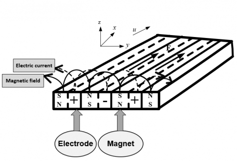
About five decades ago Gailitis and Lielausis [8] devised a Riga plate (Figure 1) which was an ingenious way to produce the wall parallel Lorentz force to control a fluid flow. This Riga plate play an important role in submarine and sheep industry. Further the Grinberg et al. [9] introduced the Grinberg term in contrast to the Hartmann number. Magyari and Pantokratoras [10] contributed a lot in investigating an aiding and opposing effects of the Lorentz force over a Riga plate with a viscous fluid flow. Hayat et al. [11] studied boundary layer flow of Nano fluid induced by a Riga plate with variable thickness. Adeel et al. [12] has investigated the steady flow of Nano fluid past Riga plate numerically. Entropy generation on viscous Nano fluid through a horizontal Riga plate for suction case has been examined by Abbas et al. [13]. This paper discussed numerical solution for Riga plate with suction velocity.

The aim of this paper is to study the unsteady one dimensional Electromagnetic boundary layer flow of a nano fluid flow along a Riga plate with suction velocity. The governing equations of the problem have been transformed by usual transformation into a non-dimensional system of partial coupled differential equations. The implicit finite difference technique has been used to solve the dimensionless system of non-linear partial differential equations. The obtained results have been shown graphically.

It is required to make the equations (1) to (5) into the dimensionless equations. The solution of the governing equations (1) to (5) under the boundary conditions (6) are based on the finite difference method. The following dimensionless variables have been used for obtaining the dimensionless governing equations.

$\begin{align}  & X=\frac{x}{l},Y=\frac{y}{L},U=\frac{u}{{{U}_{w}}},w=\frac{W}{{{U}_{w}}},\theta =\frac{T-{{T}_{\infty }}}{{{T}_{w}}-{{T}_{\infty }}}, \\  & \phi =\frac{C-{{C}_{\infty }}}{{{C}_{w}}-{{C}_{\infty }}},L=\frac{a}{\pi },l=\frac{{{U}_{w}}{{L}^{2}}}{\upsilon },\tau =\frac{t{{U}_{w}}}{l} \\ \end{align}$          (7)

The obtained dimensionless governing non-linear coupled partial differential equations are given as follows:

$\frac{\partial V}{\partial Y}\,\,=0$        (8)

$\frac{\partial U}{\partial \tau }-S\frac{\partial U}{\partial Y}=\frac{{{\partial }^{2}}U}{\partial {{Y}^{2}}}+{{R}_{c}}\theta -{{N}_{r}}\phi +{{H}_{a}}{{e}^{-Y}}+RW$                 (9)

$\frac{\partial W}{\partial \tau }-S\frac{\partial W}{\partial Y}=\frac{{{\partial }^{2}}W}{\partial {{Y}^{2}}}+{{H}_{a}}{{e}^{-Y}}-RU$           (10)

$\frac{\partial \theta }{\partial \tau }-S\frac{\partial \theta }{\partial Y}=\frac{1}{{{p}_{r}}}\frac{{{\partial }^{2}}\theta }{\partial {{Y}^{2}}}+{{N}_{b}}\frac{\partial \theta }{\partial Y}\frac{\partial \phi }{\partial Y}+{{N}_{t}}{{(\frac{\partial \theta }{\partial Y})}^{2}}$               (11)

$\frac{\partial \phi }{\partial \tau }-S\frac{\partial \phi }{\partial Y}=\frac{1}{{{L}_{e}}}\frac{{{\partial }^{2}}\phi }{\partial {{Y}^{2}}}+\frac{1}{{{L}_{e}}}\frac{{{N}_{t}}}{{{N}_{b}}}\frac{{{\partial }^{2}}\theta }{\partial {{Y}^{2}}}$                  (12)

The dimensionless boundary conditions are given as follows:

$\begin{align}  & U=0\,,\ \ W=0,\,\ \ \ \ T=1,\,\,\ \ \ \,C=1\,\,\ \ \ \ \ \ \ \ \,at\,\,Y=0 \\  & U\to 0\,,\,\ W=0\ \ \,\ \ \ T=0,\,\ \ \ \ C=0\,\,\ \ \ \ \ \ \ as\,\,\,\,Y\to \infty  \\ \end{align}$                  (13)

The non-dimensional parameters are given as follows:

Richardson number: ${{R}_{c}}=\frac{{{a}^{2}}\Delta T}{{{\pi }^{2}}\nu {{U}_{w}}}\left( 1-{{\phi }_{\infty }} \right)g{{\beta }^{*}}$, Nanoparticle concentration flux: ${{N}_{r}}=\frac{{{a}^{2}}\Delta \phi }{{{\pi }^{2}}\nu {{U}_{w}}}\frac{{{\rho }_{p}}-{{\rho }_{f}}}{{{\rho }_{f}}}$, Hartmann number: ${{H}_{a}}=\frac{1}{8\pi }\frac{{{a}^{2}}{{J}_{0}}{{M}_{0}}}{v{{U}_{w}}{{\rho }_{f}}}$, Brownian motion parameter: ${{N}_{b}}=\frac{\tau {{D}_{B}}\Delta \phi }{v}$,Lewis Number: ${{L}_{e}}=\frac{v}{{{D}_{B}}}$, Thermophoresis parameter: ${{N}_{t}}=\frac{\tau {{D}_{T}}\Delta T}{v{{T}_{\infty }}}$, Kinematic viscosity: $v=\frac{\mu }{{{\rho }_{f}}}$, Prandtl Number: ${{p}_{r}}=\frac{v}{a}$, Rotating parameter: $R=\frac{2{{a}^{2}}\Omega }{{{\pi }^{2}}\upsilon }$, Suction parameter: $S=\frac{{{v}_{0}}}{{{U}_{\infty }}}$.

3.1 Shear stress, Nusselt and Sherwood number

The quantities of chief physical interest are Shear Stress, Nusselt number, and Sherwood number. From the Primary velocity field, the effects of various parameters on the local shear stress has been investigated. The following equations represent the local shear stress at the plate.

Local shear stress,

${{\tau }_{ul}}={{R}_{{}}}{{\left( \frac{\partial U}{\partial y} \right)}_{y=0}}$                      (14)

and which are proportional to ${{\left( \frac{\partial U}{\partial y} \right)}_{y=0}}$

From the secondary velocity field, the effects of various parameters on the local shear stress have been formulated. The following equations represent the local shear stress at the plate.

Local shear stress,

${{\tau }_{wl}}={{R}_{{}}}{{\left( \frac{\partial W}{\partial y} \right)}_{y=0}}$           (15)

and which are proportional to ${{\left( \frac{\partial W}{\partial y} \right)}_{y=0}}$

From the temperature field, the effects of various parameters on the local and average heat coefficients have been formulated. The following equations represent the local and average heat transfer rate that is well known Nusselt number.

Local Nusselt number,

$N{{u}_{l}}={{\left( 1+R \right)}_{{}}}.{{\left( -\frac{\partial T}{\partial y} \right)}_{y=0}}$                          (16)

and which are proportional to ${{\left( -\frac{\partial \overline{T}}{\partial Y} \right)}_{y=0}}$

And from the concentration field, the effects of various parameter on the local mass transfer coefficients has analyzed. The following represent the local and average mass transfer rate that is well known Local Sherwood number,

$S{{h}_{l}}=.{{\left( -\frac{\partial C}{\partial y} \right)}_{y=0}}$             (17)

and which are proportional to ${{\left( -\frac{\partial \overline{C}}{\partial Y} \right)}_{y=0}}$

3.2 Numerical technique

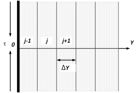
To solve the dimensionless system (8) to (13) by the implicit finite difference method subject to the boundary conditions, a set of the finite difference equation is required. For which, the region within the boundary layer is divided into a grid or mesh grid of lines perpendicular to Y axis where Y-axis is normal to the plate is as shown in Figure 3.

3.png

Figure 3. Finite difference space grid

Here it is assumed that the maximum length of the boundary layer is ${{Y}_{\max }}\left( =25 \right)$ as corresponding to$Y\to \infty $ i.e. $Y$varies from 0 to 25. The number of grid spacing $n=80$  along the $Y$directions. It is assumed that $Y$is constant mesh size $Y$directions and taken follows.

$Y=25(0\le x\le 100)$; With the smaller time-step, $\Delta \tau =0.025$

Consider  ${{U}^{'}},{{V}^{'}},{{W}^{'}},{{\theta }^{'}},{{\phi }^{'}}$ denote the values of $U,V,\theta ,\phi $ at the end of time-step respectively.

$\begin{align} & \ {{\left( \frac{\partial U}{\partial \tau } \right)}_{i,j}}=\frac{{{U}^{'}}_{j}-{{U}_{j}}}{\Delta X},{{\left( \frac{\partial U}{\partial Y} \right)}_{i,j}}=\frac{{{U}_{j+1}}-{{U}_{j}}}{\Delta Y},\,{{\left( \frac{{{\partial }^{2}}U}{\partial {{Y}^{2}}} \right)}_{i,j}}=\frac{{{U}_{j+1}}-2{{U}_{j}}+{{U}_{j-1}}}{{{(\Delta Y)}^{2}}}, \\ & {{\left( \frac{\partial W}{\partial \tau } \right)}_{i,j}}=\frac{{{W}^{'}}_{j}-{{W}_{j}}}{\Delta \tau },{{\left( \frac{\partial W}{\partial Y} \right)}_{i,j}}=\frac{{{W}_{j+1}}-{{W}_{j}}}{\Delta Y},{{\left( \frac{{{\partial }^{2}}W}{\partial {{Y}^{2}}} \right)}_{i,j}}=\frac{{{W}_{j+1}}-2{{W}_{j}}+{{W}_{j-1}}}{{{(\Delta Y)}^{2}}}, \\ & {{\left( \frac{\partial \theta }{\partial \tau } \right)}_{i,j}}=\frac{{{\theta }^{'}}_{j}-{{\theta }_{j}}}{\Delta \tau },\ {{\left( \frac{\partial \theta }{\partial Y} \right)}_{i,j}}=\frac{{{\theta }_{j+1}}-{{\theta }_{j}}}{\Delta Y}\,,{{\left( \frac{{{\partial }^{2}}\theta }{\partial {{Y}^{2}}} \right)}_{i,j}}=\frac{{{\theta }_{j+1}}-2{{\theta }_{j}}+{{\theta }_{j-1}}}{\Delta {{Y}^{2}}},\  \\ & {{\left( \frac{\partial \phi }{\partial \tau } \right)}_{i,j}}=\frac{{{\phi }^{'}}_{j}-{{\phi }_{j}}}{\Delta \tau },{{\left( \frac{\partial \phi }{\partial Y} \right)}_{i,j}}=\frac{{{\phi }_{j+1}}-{{\phi }_{j}}}{\Delta Y}\ ,\ \ {{\left( \frac{{{\partial }^{2}}\phi }{\partial {{Y}^{2}}} \right)}_{i,j}}=\frac{{{\phi }_{j+1}}-2{{\phi }_{j}}+{{\phi }_{j-1}}}{\Delta {{Y}^{2}}} \\ \end{align}$

Using the above implicit finite difference approximation the following appropriate set of finite difference equations are obtained as follows:

Momentum equation

$\frac{{{U}^{'}}_{j}-{{U}_{j}}}{\Delta t}-S(\frac{{{U}_{j+1}}-{{U}_{j}}}{\Delta Y})=\frac{{{U}_{j+1}}-2{{U}_{j}}+{{U}_{j-1}}}{{{(\Delta Y)}^{2}}}+{{R}_{c}}{{\theta }_{j}}-{{N}_{r}}{{\phi }_{j}}+{{H}_{a}}{{e}^{-Y}}+R{{W}_{j}}$              (18)

Momentum equation

$\frac{{{W}^{'}}_{i,j}-{{W}_{i,j}}}{\Delta t}-S(\frac{{{W}_{j+1}}-{{W}_{j}}}{\Delta Y})=\frac{{{W}_{j+1}}-2{{W}_{j}}+{{W}_{j-1}}}{{{(\Delta Y)}^{2}}}+{{H}_{a}}{{e}^{-Y}}-R{{U}_{j}}$            (19)

Energy equation

$\begin{align}  & \frac{{{{{\theta }'}}_{j}}-{{\theta }_{j}}}{\Delta \tau }-S(\frac{{{\theta }_{j+1}}-{{\theta }_{j}}}{\Delta Y})=\frac{1}{{{p}_{r}}}(\frac{{{\theta }_{j+1}}-2{{\theta }_{j}}+{{\theta }_{j-1}}}{{{(\Delta Y)}^{2}}}) \\ & \,\,\,\,\,\,\,\,\,\,\,\,\,\,\,\,\,\,\,\,\,\,\,\,\,\,\,\,\,\,\,\,\,\,\,\,\,\,\,\,\,\,\,\,\,\,\,\,\,\,\,\,\,\,\,\,+{{N}_{b}}(\frac{{{\theta }_{j+1}}-{{\theta }_{j}}}{\Delta Y})(\frac{{{\phi }_{j+1}}-{{\phi }_{j}}}{\Delta Y})+{{N}_{t}}{{(\frac{{{\theta }_{j+1}}-{{\theta }_{j}}}{\Delta Y})}^{2}} \\ \end{align}$            (20)

Concentration equation

$\begin{align}  & \frac{{{{{\phi }'}}_{j}}-{{\phi }_{j}}}{\Delta \tau }+U+{{V}_{i,j}}(\frac{{{\phi }_{j+1}}-{{\phi }_{j}}}{\Delta Y})=\frac{1}{{{L}_{e}}}(\frac{{{\phi }_{j+1}}-2{{\phi }_{j}}+{{\phi }_{j-1}}}{{{(\Delta Y)}^{2}}}) \\ & \,\,\,\,\,\,\,\,\,\,\,\,\,\,\,\,\,\,\,\,\,\,\,\,\,\,\,\,\,\,\,\,\,\,\,\,\,\,\,\,\,\,\,\,\,\,\,\,\,\,\,\,\,\,\,\,\,\,\,\,\,\,\,\,+\frac{1}{{{L}_{e}}}\frac{{{N}_{t}}}{{{N}_{b}}}(\frac{{{\theta }_{j+1}}-2{{\theta }_{j}}+{{\theta }_{j-1}}}{{{(\Delta Y)}^{2}}}) \\ \end{align}$         (21)

And the boundary conditions are given as follows:

$\begin{align}  & {{U}_{0}}^{n}=0,{{V}_{0}}^{n}=0,\,\,{{W}_{0}}^{n}=0,\,\,{{\theta }^{n}}_{0}=1,\,\,\,{{\phi }^{n}}_{0}=1\,\,\, \\ & {{U}_{L}}^{n}=0\,,\,{{W}_{L}}^{n}=0,\,\,\,{{\theta }^{n}}_{L}=0,\,\,{{\phi }^{n}}_{L}=0\,\,where\,\,L\to \infty \, \\ \end{align}$          (22)

Here the subscripts$j$ designate the grid points with  $y$ coordinates respectively and the subscript $n$ represents a value of time, $\tau =n\Delta \tau $ every where. From the initial condition (22), the values of $U$$W$,$\theta $ and $\phi $are known at$\tau =0$.$U$,$W$, $\theta $ and $\phi $ should eventually converge to values which are approximately the steady state solution of equations (17) to (20).

Due to analyze the physical situation of the model, the steady-state numerical values of the non-dimensional primary velocity (U), secondary velocity (W), temperature (θ) and concentration (ϕ) distributions within the boundary layer have been computed. Also, the effect on local shear stress (Primary and secondary), local Nusselt and local Sherwood number for different values of Brownian motion parameter N_b, Thermophoresis parameter N_t, Lewis number L_e, Richardson number R_c, Suction parameter S and Rotation parameter R have been shown graphically.

5.1 Mesh sensitivity and code validation tests

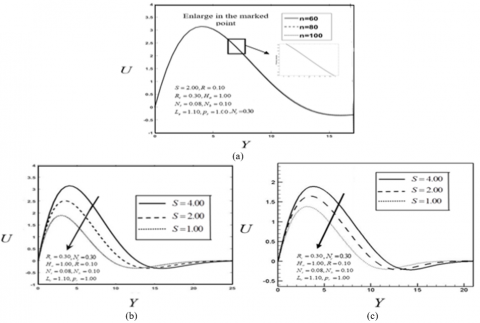
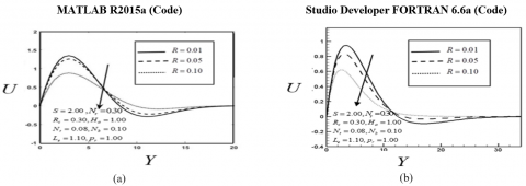
To verify the effects of grid space for n, the computations have been carried out for three different grid spaices such as n=60; n=80 and n=100 are shown in Figure 4(a). But negligible changes have been seen among these graphs. According to this situation, the results of primary velocity, secondary velocity, temperature and distributions have been carried out for n=80. The computations have been carried out by using MATLAB R2015a code and Studio Developer FORTRAN 6.6a (SDF) code. The results of both codes are qualitatively same but not and quantitatively which are shown in Figures 4(b,c). From these figures, the same results have been occurred on primary velocity for different values of suction parameters which have been shown for the results of both codes.

5.2 Time sensitivity test (steady state solution)

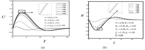
To obtain the steady-state solution, the computations have been carried out for different time step sizes such as τ=5.0, 10.0, 20.0, 40.0, 50.0, and 60.0. It is observed that the result of computations for different time distributions, however, shows little changes after τ=20.0. Thus the solutions for τ=40.0 are taken essentially as the steady-state solutions. The time variation for primary (U), secondary velocity (W), temperature (θ) and concentration (ϕ) distributions are shown in Figures 5 to 6.

5.3 Validation test (comparison)

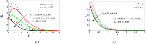
A qualitative and quantitative comparisons of the present steady-state results with the published results of Abaas et al. [13] are presented in Figure 7. Thus, the present results and the published results of Abaas et al. [13] are qualitatively quite same.

Figure $7(\mathrm{a})$ The effect of Brownian motion $N_{b}$ parameter and Prandtl's number $p_{r}$ on Concentration distribution of the present study without Rotation parameter. And (b) The effect of Brownian motion $N_{b}$ parameter and Prandtl's number $p_{r}$ on Concentration distribution of Abbas et al. [13].

5.4 Effects of different parameters on velocity distribution, temperature distribution, and concentration distribution

In order to get the clear concept of physical properties of the problem, the effects of different parameters namely Rotation parameter R, Richardson parameter R_c, Suction parameter S, Brownian motion parameter N_b, Thermophoresis parameter N_t, Lewis number L_eare presented graphically. For numerical computations, it has been used S=2.00 N_r=0.30, R_c=1.00, R=0.10, H_a=1.00, N_t=0.08, N_b=0.10, L_e=1.10, p_r=1.00 arbitrarily.

The effects of Rotation parameter R on Primary velocity is shown in Figure 8. It is observed from Figure 8 that the primary velocity decreases with the increase of the Rotation parameter R. On the other hand secondary velocity increases with the increase of the Rotation parameter R which are shown in Figure 9. It is observed from Figure 10 that the primary velocity increases with the increase of Richardson parameter R_cwhile secondary velocity decreases with the increase of Richardson parameter R_c which are shown in Figure 11. Also, it is seen from Figure 10 and Figure 11 that the boundary layer growth of primary velocity is weaker than secondary velocity.

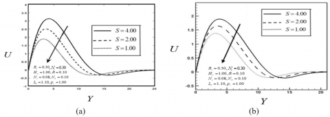
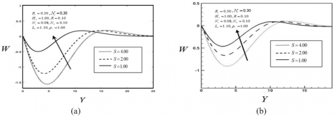
The effects of Suction parameter S on primary velocity are shown in Figure 12. It is observed that primary velocity decreases with the decrease of Suction parameter S. The Figure 13 displays that the secondary velocity increases with the decrease of Suction parameter S.

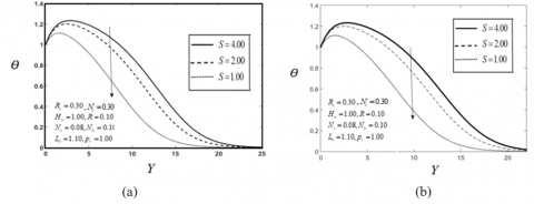
Figure 14 shows that temperature distribution for different values of Suction parameter S, the temperature gradually decreases with the increase of Suction parameter S.

The effects of Brownian motion parameter N_b on Temperatur distribution increases in Figure 15. It is observed that temperature distribution increases with the increase of Brownian motion parameter N_b

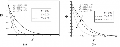
The effects of Suction parameter S on Concentration distribution decreases in Figure 16. It is observed from this figure that Concentration distribution decreases with the increase of Suction parameter S.

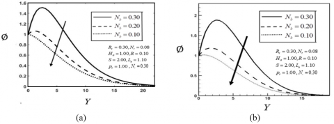
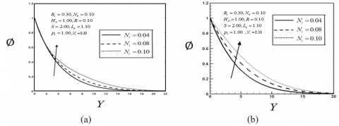
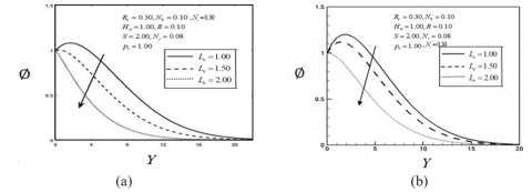
In Figure 17, Concentration distribution is decreases with the decrease of Brownian motion parameter N_b. Figure 18 displays the effects of Thermophoresis parameter N_t on Concentration distribution. It is seen that Concentration distribution increases with the increase of Thermophoresis motion parameter N_t. Figure 19 shows the concentration distribution for different values of Lewis number L_e, while Concentration distribution decreases with the increase of Lewis number L_e.

4.png

Figure 4. Justification of grid space for (a) primary velocity (MATLAB R2015a). Effect of Suction parameter S for (b) primary velocity (MATLAB R2015a) and (c) primary velocity (Studio Developer FORTRAN 6.6a)

5.png

Figure 5. Illustration of time variation for (a) primary velocity and (b) secondary velocity

6.png

Figure 6. Illustration of time variation for (a) Temperature distribution and (b) Concentration distribution

7.png

Figure 7. Comparison between steady-state results and the published results

8.png

Figure 8. Effect of Rotation parameter R for (a) primary velocity (MATLAB R2015a) and (b) Primary velocity (Studio Developer FORTRAN 6.6a)

9.png

Figure 9. Effect of Rotation parameter R for (a) Secondary velocity (MATLAB R2015a) and (b) Secondary velocity (Studio Developer FORTRAN 6.6a)

10.png

Figure 10. Effect of Richardson number R_c for (a) primary velocity (MATLAB R2015a) and (b) Primary velocity (Studio Developer FORTRAN 6.6a)

11.png

Figure 11. Effect of Richardson number R_c for (a) Secondary velocity (MATLAB R2015a) and (b) Secondary velocity (Studio Developer FORTRAN 6.6a)

12.png

Figure 12. Effect of Suction parameter S for (a) primary velocity (MATLAB R2015a) and (b) Primary velocity (Studio Developer FORTRAN 6.6a)

13.png

Figure 13. Effect of Suction parameter S for (a) Secondary velocity (MATLAB R2015a) and (b) Secondary velocity (Studio Developer FORTRAN 6.6a)

14.png

Figure 14. Effect of Suction parameter S for (a) Temperature distribution (MATLAB R2015a) and Temperature distribution (Studio Developer FORTRAN 6.6a)

15.png

Figure 15. Effect of Brownian motion parameter N_b for (a) Temperature distribution (MATLAB R2015a) and (b) Temperature distribution (Studio Developer FORTRAN 6.6a)

16.png

Figure 16. Effect of Suction parameter S for (a) Concentration distribution (MATLAB R2015a) and (b) Concentration distribution (Studio Developer FORTRAN 6.6a)

17.png

Figure 17. Effect of Brownian motion parameter N_b for (a) Concentration distribution (MATLAB R2015a) and (b) Concentration distribution (Studio Developer FORTRAN 6.6a)

18.png

Figure 18. Effect of Thermophoresis parameter N_t for (a) Concentration distribution (MATLAB R2015a) and (b) Concentration distribution (Studio Developer FORTRAN 6.6a)

19.png

Figure 19. Effect of Lewis number L_e for (a) Concentration distribution (MATLAB R2015a) and (b)Concentration distribution (Studio Developer FORTRAN 6.6a)

5.5 Effects of different parameters on local shear stress, local Nusselt number, and local Sherwood number

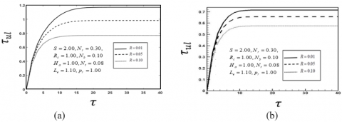
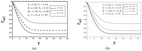
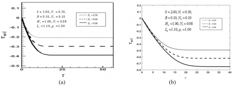
It is observed from Figs. 20 and 21 that the effects of Rotation parameter $R$on primary local shear stress  decreases gradually for decreasing the values of Rotation parameter $R$ while the effects of Rotation parameter $R$on Secondary local shear stress  increases for decreasing the values of Rotation parameter $R$. It is seen from the figures, the primary local shear stress have strong decreasing effect while the secondary local shear stress have weak increasing effect.

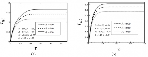
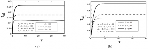
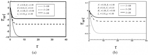
The effects of Richardson number ${{R}_{c}}$on Primary and secondary local shear stress are shown in Figs22 and 23. From the figures it is observed that primary local shear stress  increases with the increase of Richardson number ${{R}_{c}}$ while the Secondary local shear stress  decreases with the increase of Richardson number ${{R}_{c}}$. It is seen from the figures, the secondary local shear stress have strong decreasing effect while the primary local shear stress have weak increasing effect. The effects of Suction parameter $S$ on Primary and secondary local shear stress are shown in Figs24 and 25. From these figures it is observed that primary local shear stress decreases with the decrease of the Suction parameter $S$while the Secondary velocity, secondary local shear stress increases with the increase of Suction parameter $S$. It is seen from the figures, the secondary local shear stress have strong decreasing effect while the primary local shear stress have weak increasing effect.

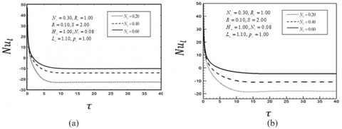
It is observed from Fig. 26 that the effect of Brownian motion parameter ${{N}_{b}}$on local Nusselt number  increases with the increase of Brownian motion parameter ${{N}_{b}}$. The effect of Thermoporasis motion parameter ${{N}_{t}}$ on the local Nusselt number  decreases with the increase of Thermoporasis motion parameter ${{N}_{t}}$which is shown in Fig. 27. The effect of Suction parameter  $S$ on Sherwood number decreases for increasing  the values of Suction parameter  $S$.

20.png

Figure 20. Effect of Rotation parameter R for (a) primary local shear stress (MATLAB R2015a) and (b) Primary local shear stress (Studio Developer FORTRAN 6.6a)

21.png

Figure 21. Effect of Rotation parameter R for (a)) Secondary local shear stress (MATLAB R2015a) and (b) Secondary local shear stress (Studio Developer FORTRAN 6.6a)

22.png

Figure 22. Effect of Richardson number R_c for (a) Primary local shear stress (MATLAB R2015a) and (b) Primary local shear stress (Studio Developer FORTRAN 6.6a)

23.png

Figure 23. Effect of Richardson number R_c for (a) Secondary local shear stress (MATLAB R2015a) and (b) Secondary local shear stress (Studio Developer FORTRAN 6.6a)

24.png

Figure 24. Effect of Suction parameter S for (a) Primary local shear stress (MATLAB R2015a) and (b) Primary local shear stress (Studio Developer FORTRAN 6.6a)

25.png

Figure 25. Effect of Suction parameter S for (a) Secondary local shear stress (MATLAB R2015a) and (b)Secondary local shear stress (Studio Developer FORTRAN 6.6a)

26.png

Figure 26. Effect of Browninan motion parameter N_b for (a) local Nusselt number (MATLAB R2015a) and (b) local Nusselt number (Studio Developer FORTRAN 6.6a)

27.png

Figure 27. Effect of Thermophoresis parameter N_t for (a) local Nusselt number (MATLAB R2015a) and (b) local Nusselt number (Studio Developer FORTRAN 6.6a)

28.png

Figure 28. Effect of Suction parameter S for (a) local shearwood number (MATLAB R2015a) and (b) local shearwood number (Studio Developer FORTRAN 6.6a)