Bekrar Lyas* | Omar Bouhali | Saad Khadar | Yaichi Mohammed
OPEN ACCESS
This paper proposes a novel dual three-phase Space Vector Modulation (SVM) for six-phase multilevel inverter to control a Six Phase Induction Machine (SPIM). The main idea is to control the six-phase multilevel inverter as two three-phase (1, 3 and 5 phases for the first one and 2, 4 and 6 phases for the second one) multilevel inverters separately by SVM of the N-level three-phase Separate DC Source (SDCS) inverter. This enables a great the simplification of the control algorithm for six phase multilevel (N level) inverter drive. In Six-Phase SVM, N6 vectors are used so if two level N=2, 3 level or 4 level, implies 64 vectors, 729 vectors, 15625 vectors are used respectively. However, in a proposed dual three-phase SVM, we use N3 vectors so if 2 level, 3 level or 4 level implies 8 vectors, 27 vectors, 125 vectors are used respectively to control the six-phase multilevel inverters as two three-phase multilevel inverter with the same three-phase multilevel SVM. Whereas the first three-phase inverter is composed by 1, 3, and 5 phases and the second three-phase is composed by 2, 4 and 6 phases. This allows to have a new modulation technique for six-phase multi-level inverter and a great simplification of the classical six-phase SVM control algorithm. The simulation results of the Indirect Field Oriented Control (IFOC) of six-phase induction machine drive fed by stacked multilevel inverters are given to highlight the performance of the proposed control structure.
dual three-phase induction machine, multi-phase machine, multilevel inverter, space vector modulation
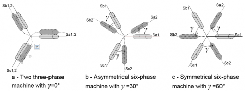
During the last decade, the use of multi-phase motor drives in high reliability application has substantially increased because of their potential advantages [1, 2]. This rapid surge concerns specifically three particular applications zones: electric ship impetus, “more electric” flying machine, and footing (locomotive, electric vehicles and hybrid electric vehicles) [3]. Two distinct features make multi-phase drives an attractive possibility for these applications. There are three possible winding connections of the six-phase machine structures (see Figure 1). In the most famous abundant one, two three-phase IM shifted by $\gamma=0^{\circ}$ (Figure 1(a)), asymmetrical six-phase machine, stator winding is composed of two three-phase windings shifted in space by $\gamma=30^{\circ}$ (Figure 1(b)). In the other structure, symmetrical six-phase machine, there are two sets of three-phase windings that are spatially shifted by $\gamma=60^{\circ}$ (Figure 1(c)), giving rise to spatial displacement between any two successive phases of 60° [3, 6].
The asymmetrical six-phase machine is the customary choice, predominantly for historical reasons associated with PWM of Voltage-Source Inverter (VSI) control [4, 6]. This allows a good quality of the current regulation which can be linked to a PWM regulation method suitable for VSI Control at a sufficiently high switching frequency 3xn (n: number of phase) [7, 8]. The asynchronous machines with numbered phases do not have the shape 3xn. For instance, five or seven [9, 10] are infrequently used in practice because they made on demand. On the other hand, the machines with six or nine phases can be gotten two or three available three-phase IM respectively. This uses the original frame and stratifications stator/rotor of the machines with three-phase and thus allows saving on the making’s cost.
Multilevel converters are able to generate output voltage wave forms consisting of a large number of steps. In this way, high voltages can be synthesized using sources and switching devices with lower voltage values, with the additional benefit of a reduced harmonic distortion and lower dv/dt in the output voltages [11, 12]. Multilevel inverter supplied multi-phase drives have been gaining the interest of researchers and industry in recent years [1, 6]. Multi-level multi-phase inverter topologies have been widely recognized as a viable solution to overcome current and voltage limits of power switching converters in the environment of high-power medium-voltage drive systems [13, 15]. Several studies published the news PWM modulations methods that can be used in multi-phase applications with several levels [16-19]. The first successful implementation of an algorithm of multi-phase SVPWM with several levels based on the approach SVM [20-26]. Such an approach is considered like a classical approach SVPWM presented in [18]. This presents a general space-vector modulation algorithm for three-level inverter. The algorithm is to a great extent computationally proficient and independent of the number of converter levels. At the same time, it provides a good insight into the operation of multilevel inverters.
Figure 1. Winding connection of six-phase machine
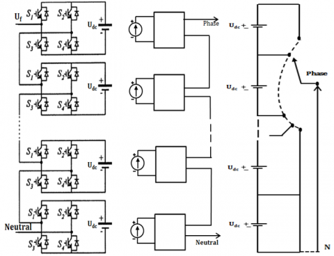
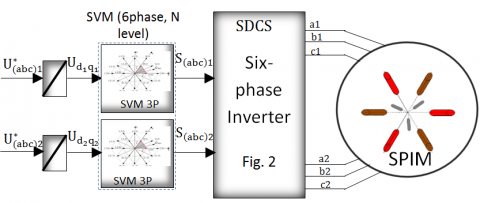
In This paper, a novel dual three-phase SVM for a multilevel inverter six-phase is proposed to drive a six-phase induction machine. The pth phase (p=1, 2, 3, 4, 5, and 6) of the six-phase multilevel SDCS inverter is shown in Figure 2. The main idea is to use the six-phase inverter as two three-phase inverter (p=1, 3, 5) and (p=2, 4, 6) to control the SPIM as two three-phase IM (U135 and U246) separately. The two multilevel three-phase inverter SDCS is controlled by two conventional N level three-phase SVM [20]. The first one can control the phases 1, 3, and 5 (Ua1b1c1), and the second one can control the phase 2, 4, and 6 (Ua2b2c2), according to the type of the six-phase machine with placed windings (two three-phase induction machine, asymmetric six-phase or symmetrical respectively). Usually, in SVM of six-phase inverter, we use N6 vectors; (for N=2, 3, or 4; there are 64 vectors, 729 vectors or 15625 vectors, respectively), and several transformations and decomposition in two plans. However, in the proposed dual SVM, we use N3 vectors; (for N=2, 3 or 4; there are 8 vectors, 27 vectors or 125 vectors respectively) in order to control two multilevel six-phase inverters.
This paper consists of six sections. The first section provides the description and model of the dual stator induction machine in the abc plan. The second section deals with Park’s SPIM model. The third section presents the developed multilevel dual three-phase SVM. As for the fourth section, it is devoted to the presentation of indirect field oriented control. The simulation results are discussed in section five, followed by a conclusion in the last section.
Figure 2. General Structure of a multilevel pth phase (p=1… 6) SDCS inverter
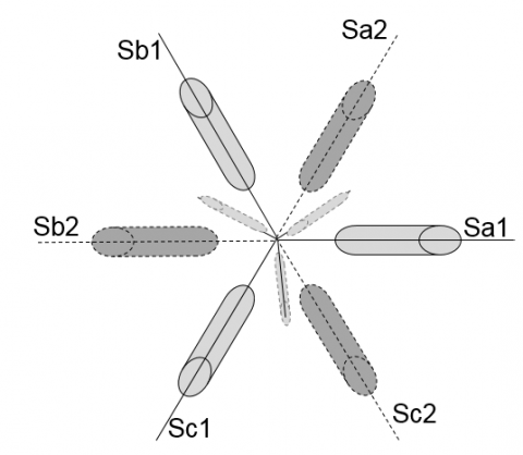
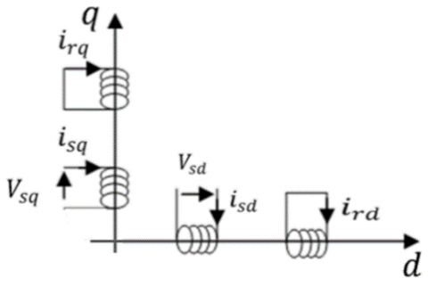
All SPIM are strictly being investigated for various high power applications due to their augmented power to weight ratio, augmented frequency and abridged magnitude of torque pulsation, and fault tolerant characteristics. The SPIM with two similar stator three phase windings, shifted by 0, 30, 60 degrees in space and three phase winding in rotor is shown in Figure 3. To put it simply, we will consider that the electrical circuit of the rotor is equivalent to a three-phase winding short-circuit [27, 28]. Figure 3 gives the position of the magnetic axes of the nine windings forming the six phases of the stator and the three phases of the rotor.
Figure 3. Stator and rotor windings of the SPIM for $\gamma=0^{\circ}, 30^{\circ}$ or $60^{\circ}$
2.1 Electrical equation
Electrical equations of the stator, rotor, electromagnetic torque (1-3) and mechanical equations (4) are expressed as a function of the different currents and the derivative of the flux. These differential equations defined in the real reference frame abc, are written as follows:
The voltage and flux linkage equations are given compactly in matrix form as:
$\left\{\left[\begin{array}{l}{\left[\mathrm{V}_{\mathrm{s}}\right]} \\ {\left[\mathrm{V}_{\mathrm{r}}\right]}\end{array}\right]=\left[\begin{array}{c}{\left[\mathrm{R}_{\mathrm{s}}\right][0]_{6 \times 3}} \\ {[0]_{3 \times 6}\left[\mathrm{R}_{\mathrm{r}}\right]}\end{array}\right]\left[\begin{array}{l}{\left[\mathrm{i}_{\mathrm{s}}\right]} \\ {\left[\mathrm{i}_{\mathrm{r}}\right]}\end{array}\right]+\frac{\mathrm{d}}{\mathrm{dt}}\left[\begin{array}{l}{\left[\varphi_{\mathrm{s}}\right]} \\ {\left[\varphi_{\mathrm{r}}\right]}\end{array}\right]\right.$ (1)
$\left[\begin{array}{l}{\left[\varphi_{s}\right]} \\ {\left[\varphi_{r}\right]}\end{array}\right]=\left[\begin{array}{l}{\left[L_{s}\right]\left[M_{s r}\right]} \\ {\left[M_{r s}\right]\left[L_{r}\right]}\end{array}\right] \cdot\left[\begin{array}{l}{\left[i_{s}\right]} \\ {\left[i_{r}\right]}\end{array}\right]$ (2)
2.2 Electromagnetic torque equation
The electromagnetic torque can be expressed in the following equations:
$\left[C_{e}\right]=\left[i_{s}\right]^{t} \frac{\left[M_{r s}\right]}{d \theta}\left[i_{r}\right]$ (3)
2.3 Mechanical equation
$\frac{\left[\Omega_{m}\right]}{d t}=\frac{1}{J}\left(C_{e}-C_{r}\right)$ (4)
With:
$\left[V_{s}\right]=\left[\begin{array}{l}{\left[V_{s, a b c 1}\right]} \\ {\left[V_{s, a b c 2}\right]}\end{array}\right] ;\left[i_{s}\right]=\left[\begin{array}{l}{\left[i_{s, a b c 1}\right]} \\ {\left[i_{s, a b c 2}\right]}\end{array}\right]$
$\left[\varphi_{s}\right]=\left[\begin{array}{l}{\left[\varphi_{s, a b c 1}\right]} \\ {\left[\varphi_{s, a b c 2}\right]}\end{array}\right] ;\left[V_{r}\right]=\left[V_{r, a b c}\right] ;\left[i_{r}\right]=\left[i_{r, a b c}\right]$
$\left[R_{s}\right]=\left[\begin{array}{c}{\left[R_{s 1}\right][0]_{3 \times 3}} \\ {[0]_{3 \times 3}\left[R_{s 2}\right]}\end{array}\right] ;\left[\varphi_{s}\right]=\left[\left[\begin{array}{c}{\left[\varphi_{s, a b c 1}\right]} \\ {\left[\varphi_{s, a b c 2}\right]}\end{array}\right]\right.$
$\left[L_{s}\right]=\left[\begin{array}{l}{\left[L_{s 1, s 1}\right]\left[M_{s 1, s 2}\right]} \\ {\left[M_{s 2, s 1}\right]\left[L_{s 2, s 2}\right]}\end{array}\right] ;\left[M_{s r}\right]=\left[\begin{array}{l}{\left[M_{s 1, r}\right]} \\ {\left[M_{s 2, r}\right]}\end{array}\right]$
$\left[M_{r s}\right]=\left[M_{s r}\right]^{t} ;\left[M_{s 1, s 2}\right]=\left[M_{s 2, s 1}\right]^{t}$
After the replacement of the stator and rotor flows and the different inductances in equation (2), we obtain [21]:
$\left[\begin{array}{c}\varphi_{s, a b c 1} \\ \varphi_{s, a b c 2} \\ \varphi_{r, a b c}\end{array}\right]=\left[\begin{array}{ccc}L_{s 1, s 1} & M_{s 1, s 2} & M_{s 1, r} \\ M_{s 2, s 1} & L_{s 2, s 2} & M_{s 2, r} \\ M_{r, s 1} & M_{r, s 2} & L_{r, r}\end{array}\right]\left[\begin{array}{c}i_{s, a b c 1} \\ i_{s, a b c 2} \\ i_{r, a b c}\end{array}\right]$ (5)
where, $\left[\mathrm{v}_{\mathrm{s}}\right],\left[\mathrm{i}_{\mathrm{s}}\right],\left[\mathrm{v}_{\mathrm{r}}\right],\left[\mathrm{i}_{\mathrm{r}}\right],\left[\varphi_{\mathrm{s}}\right]$ are the stator and rotor voltage, current and flux vectors of the six-phase IM. We find that the machine six-phase is composed of two times the machine three-phase asynchronous. This allows for the study and synthesis of control laws of two three-phase induction machines using the methods already developed instead of ordering directly the six phase machine. In the next part, we will present Park's transformation, which leads to a simplified model of SPIM that is easy to solve and more suitable for the study of dynamic regimes and control.
Two park models are presented. The first obtained by transforming the stator voltages (6/2x3) is used for the SVM control. The second is obtained for a transformation (6/2) that will be used as a two-phase system for Indirect Field Oriented Control.
3.1 Dual three-phase model of stator voltages
In this section, the association of two three-phase machines. By applying the Park transformation of the two-stator stars, we obtain twice the two-phase models equivalent to the three-phase model (Figure 4) [28, 29]. In which we use for this the usual transformation of Concordia and Park.
$\left\{\begin{array}{c}X_{(\alpha \beta 0) i}=[T]^{-1} X_{(a b c) i} \\ X_{(d q 0) i}=[\rho(\theta)]^{-1} X_{(\alpha \beta 0) i}\end{array}\right.$ (6)
where, X can represent the current, the voltage or the flux in the machine, and i can represent 1 for the first stator and 2 for the second stator.
with:
$[T]^{-1}=\sqrt{\frac{2}{3}}\left[\begin{array}{ccc}\cos (0) & \cos \left(\frac{2 \pi}{3}\right) & \cos \left(\frac{4 \pi}{3}\right) \\ \sin (0) & \sin \left(\frac{2 \pi}{3}\right) & \sin \left(\frac{4 \pi}{3}\right) \\ \frac{1}{\sqrt{2}} & \frac{1}{\sqrt{2}} & \frac{1}{\sqrt{2}}\end{array}\right]$ (7)
$[\rho(\theta)]^{-1}=\left[\begin{array}{ccc}\cos (\theta) & \sin (\theta) & 0 \\ -\sin (\theta) & \cos (\theta) & 0 \\ 0 & 0 & 1\end{array}\right]$ (8)
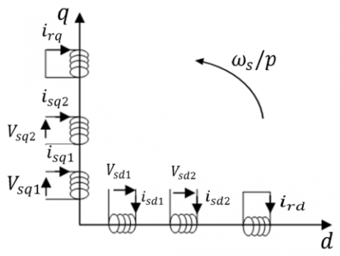
Figure 4. Representation of the SPIM windings in the Park
By applying the Park transformation (6) to the equations of the voltages (1), the real equation system of the SPIM will be decomposed into two diphasic subsystems (d1-q1) and (d2-q2).
$\left\{\begin{array}{l}V_{s d i}=R_{s} I_{s d i}+\frac{d \varphi_{s d i}}{d t}-\omega_{s} \varphi_{s q i} \\ V_{s q i}=R_{s} I_{s q i}+\frac{d \varphi_{s q i}}{d t}+\omega_{s} \varphi_{s d i} \\ V_{s o i}=R_{s} I_{s o i}+\frac{d \varphi_{s o i}}{d t}\end{array}\right.$ (9)
with: (i=1 or 2)
This shows that we have two stators, and the voltages are decoupled [32]. This property of the stator voltages will operate to use two SVM, each one will control three phases separately.
3.2 Six-phase model in the system (d, q) (x, y) (o1, o2)
In this section, a bi-phase command model of SPIM is presented. Therefore, the matrix of stator inductors [Ls] is diagonalized by the stator decoupling matrix $\left[\mathrm{T}_{\mathrm{s}}(\gamma)\right]^{-1}$ [30], [31] and the rotor matrix [Tr]-1 is follow:
$\left[T_{s}(\gamma)\right]^{-1}=\frac{1}{\sqrt{3}}\left[\begin{array}{cccccc}\cos (0) &\cos \left(\frac{2 \pi}{3}\right) &\cos \left(\frac{4 \pi}{3}\right)& \cos (\gamma) & \cos \left(\gamma+\frac{2 \pi}{3}\right) &\cos \left(\gamma+\frac{4 \pi}{3}\right) \\ \sin (0) &\sin \left(\frac{2 \pi}{3}\right) &\sin \left(\frac{4 \pi}{3}\right) &\sin (\gamma) & \sin \left(\gamma+\frac{2 \pi}{3}\right) &\sin \left(\gamma+\frac{4 \pi}{3}\right) \\ \cos (0) &\cos \left(\frac{4 \pi}{3}\right) &\cos \left(\frac{2 \pi}{3}\right) &\cos (\pi-\gamma) &\cos \left(\frac{\pi}{3}-\gamma\right) &\cos \left(\frac{5 \pi}{3}-\gamma\right) \\ \sin (0) &\sin \left(\frac{4 \pi}{3}\right)& \sin \left(\frac{2 \pi}{3}\right) &\sin (\pi-\gamma) & \sin \left(\frac{\pi}{3}-\gamma\right) &\sin \left(\frac{5 \pi}{3}-\gamma\right) \\ 1 & 1&1&0&0&0 \\ 0 & 0 & 0&1&1&1\end{array}\right]$ (10)
$[T r]^{-1}=\sqrt{\frac{2}{3}}\left[\begin{array}{ccc}1 & -\frac{1}{2} & -\frac{1}{2} \\ 0 & \frac{\sqrt{3}}{2} & -\frac{\sqrt{3}}{2} \\ \frac{1}{\sqrt{2}} & \frac{1}{\sqrt{2}} & \frac{1}{\sqrt{2}}\end{array}\right]$ (11)
with, $\gamma=0^{\circ} ; 30^{\circ} ;$ or $60^{\circ}$ two three-phase induction machine, asymmetric six-phase or symmetrical SPIM respectively. By applying the transformation matrix $\left[\mathrm{T}_{\mathrm{s}}(\gamma)\right]^{-1}$ to the equations of voltages (1) and fluxes (2), the system of real six-dimensional stator equations will be decomposed into three decoupled subsystems of dimension two: the systems (d-q), (x-y) et (o1-o2). Geometrically, we will "project" the stator variables on three orthogonal "planes". The transformation matrix has the property of separating the harmonics into several groups, and projecting them into each subsystem. For rotor variables, the usual Concordia transformation, denoted by [Tr]-1 (11), is used. (See Figure 5).
Figure 5. Equivalent model of SPIM in (d-q) plan
By applying the transformation matrix (10) to equation (2) the system becomes:
$\left[\begin{array}{c}\varphi_{s d} \\ \varphi_{s q} \\ \varphi_{s x} \\ \varphi_{s y} \\ \varphi_{s o 1} \\ \varphi_{s o 2}\end{array}\right]=\left[\begin{array}{cccccc}L_{s} & 0 & 0 & 0 & 0 & 0 \\ 0 & L_{s} & 0 & 0 & 0 & 0 \\ 0 & 0 & L_{s 1} & 0 & 0 & 0 \\ 0 & 0 & 0 & L_{s 1} & 0 & 0 \\ 0 & 0 & 0 & 0 & L_{s 1} & 0 \\ 0 & 0 & 0 & 0 & 0 & L_{s 1}\end{array}\right]\left[\begin{array}{c}i_{s d} \\ i_{s q} \\ i_{s x} \\ i_{s y} \\ i_{s o 1} \\ i_{s o 2}\end{array}\right]+M\left[\begin{array}{cccc}\cos \theta_{r, s} & -\sin \theta_{r, s} & 0 & \\ \sin \theta_{r, s} & \cos \theta_{r, s} & 0 & \\ 0 & 0 & 0 \\ 0 & 0 & 0 \\ 0 & 0 & 0 \\ 0 & 0 & 0\end{array}\right]\left[\begin{array}{c}i_{r d} \\ i_{r q} \\ i_{r 0}\end{array}\right]$ (12)
$\left[\begin{array}{c}\varphi_{r d} \\ \varphi_{r d} \\ \varphi_{r 0}\end{array}\right]=M\left[\begin{array}{ccc}{\left[\begin{array}{cc}\cos \theta & \sin \theta \\ -\sin \theta & \cos \theta\end{array}\right]} & {[0]_{2 * 4}} \\ {[0]_{1 * 4}} & {[0]_{4 * 4}}\end{array}\right]\left[\begin{array}{c}i_{s d}\\i_{s q} \\ i_{s x} \\ i_{s y} \\ i_{s 01} \\ i_{s 02}\end{array}\right]+\left[\begin{array}{ccc}L_{r} & 0 & 0 \\ 0 & L_{r} & 0 \\ 0 & 0 & L_{r 1}\end{array}\right]\left[\begin{array}{c}i_{r d} \\ i_{r q} \\ i_{r 0}\end{array}\right]$ (13)
The next step is to eliminate the dependence of θ of the matrix of inductances. For this, we use a rotation matrix [⍴(θ)] to express the rotor variables in the stator reference:
$\left\{\begin{array}{l}X_{\alpha \beta 0}=\left[T_{s}(\gamma)\right]^{-1} X_{a b c} \\ X_{d q 0}=[\rho(\theta)]^{-1} X_{\alpha \beta 0}\end{array}\right.$ (14)
where, X can represent the current, the voltage, or the flux in the six-phase machine, dq xy 01 01.
with:
$[\rho(\theta)]^{-1}=\left[\begin{array}{ccc}{\left[\begin{array}{cc}\cos \theta & \sin \theta \\ -\sin \theta & \cos \theta\end{array}\right]} & {[0]_{2 * 4}} \\ {[0]_{4 * 2}} & {[0]_{4 * 4}}\end{array}\right]$ (15)
where the models are:
We use the common Park transformation matrix for the rotor size.
$\left[\begin{array}{c}x_{\mathrm{sc}} \\ x_{s \beta} \\ x_{\mathrm{sx}} \\ x_{\mathrm{sy}} \\ x_{\mathrm{so1}} \\ x_{\mathrm{so} 2}\end{array}\right]=\left[T_{s}(\gamma)\right]^{-1}\left[\begin{array}{c}x_{\mathrm{sa} 1} \\ x_{\mathrm{sb} 1} \\ x_{\mathrm{sc} 1} \\ x_{\mathrm{sa} 2} \\ x_{\mathrm{sb} 2} \\ x_{\mathrm{sc} 2}\end{array}\right]$ (16)
$\left[x_{r \alpha} x_{r \beta} x_{r o}\right]^{t}=\left[T_{r}\right]^{-1}\left[x_{r a} x_{r b} x_{r c}\right]^{t}$ (17)
$\left[T_{r}\right]^{-1}=\sqrt{\frac{2}{3}}\left[\begin{array}{ccc}\cos (0) & \cos \left(\frac{2 \pi}{3}\right) & \cos \left(\frac{4 \pi}{3}\right) \\ \sin (0) & \sin \left(\frac{2 \pi}{3}\right) & \sin \left(\frac{4 \pi}{3}\right) \\ \frac{1}{\sqrt{2}} & \frac{1}{\sqrt{2}} & \frac{1}{\sqrt{2}}\end{array}\right]$ (18)
By expressing the model of the SPIM in a reference linked to the stator, we obtain:
$\left[\begin{array}{c}V_{s \alpha} \\ V_{s \beta} \\ V_{r \alpha} \\ V_{r \beta}\end{array}\right]=\left[\begin{array}{cccc}r_{s} & 0 & 0 & 0 \\ 0 & r_{s} & 0 & M \\ 0 & \omega M & r_{r} & \omega L_{r} \\ -\omega M & 0 & -\omega L_{r} & r_{r}\end{array}\right]\left[\begin{array}{c}i_{s \alpha} \\ i_{s \beta} \\ i_{r \alpha} \\ i_{r \beta}\end{array}\right]+\left[\begin{array}{cccc}L_{s} & 0 & M & 0 \\ 0 & L_{s} & 0 & M \\ M & 0 & L_{r} & 0 \\ 0 & M & 0 & L_{r}\end{array}\right] \frac{d}{d t}\left[\begin{array}{c}i_{s \alpha} \\ i_{s \beta} \\ i_{r \alpha} \\ i_{r \beta}\end{array}\right]$ (19)
$\left[\begin{array}{l}\mathrm{V}_{\mathrm{sx}} \\ \mathrm{V}_{\mathrm{sy}}\end{array}\right]=\left[\begin{array}{ll}\mathrm{r}_{\mathrm{s}} & 0 \\ 0 & \mathrm{r}_{\mathrm{s}}\end{array}\right]\left[\begin{array}{l}\mathrm{i}_{\mathrm{sx}} \\ \mathrm{i}_{\mathrm{sy}}\end{array}\right]+\left[\begin{array}{ll}\mathrm{L}_{\mathrm{s} 1} & 0 \\ 0 & \mathrm{L}_{\mathrm{s} 1}\end{array}\right] \frac{\mathrm{d}}{\mathrm{dt}}\left[\begin{array}{l}\mathrm{i}_{\mathrm{sx}} \\ \mathrm{i}_{\mathrm{sy}}\end{array}\right]$ (20)
$\left[\begin{array}{c}V_{s o 1} \\ V_{s o 2} \\ V_{r o}\end{array}\right]=\left[\begin{array}{ccc}r_{s} & 0 & 0 \\ 0 & r_{s} & 0 \\ 0 & 0 & r_{r}\end{array}\right]\left[\begin{array}{c}i_{s 01} \\ i_{s 02} \\ i_{r o}\end{array}\right]+\left[\begin{array}{ccc}L_{s 1} & 0 & 0 \\ 0 & L_{s 1} & 0 \\ 0 & 0 & L_{r 1}\end{array}\right] \frac{d}{d t}\left[\begin{array}{c}i_{s 01} \\ i_{s o 2} \\ i_{r 0}\end{array}\right]$ (21)
The mechanical equation and electromagnetic torque are as follows:
$C_{e m}=p . M\left(i_{s \beta} i_{r \alpha}-i_{s \alpha} i_{r \beta}\right)$
$C_{e m}-C_{r}-K_{f} \Omega_{m}=J_{1} \frac{d \Omega_{m}}{d t} ; \frac{d \theta}{d t}=\Omega_{m}$ (22)
where, J1 denotes the moment of inertia of the six-phase machine and Cr the resistive torque.
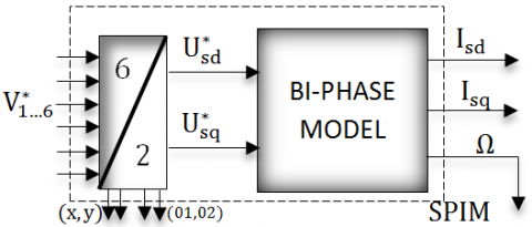
We note that the new SPIM model has three completely decoupled sub-models (d-q), (x-y) and (o1-o2). The sub-model (d-q) is exactly similar to that of a three-phase asynchronous machine whose variables are responsible for the electromechanical conversion of energy in the SPIM. On the other hand, the equations of the sub-model (x-y) are totally decoupled from the other equations, and in particular from the rotor equations. The variables in this subsystem represent the circulation currents in the SPIM and therefore do not contribute to the electromechanical conversion of the energy. Finally, the subsystem (o1-o2) which contains the classical homopolar components [30]. We saw previously that the electromechanical conversion of the energy is only related to the two components isd, isq, for that we will interest only to the reference (d-q), in which the six quantities of the SPIM will be represented by two sizes equivalents in quadrature, and which called bi-phase control model. The SPIM model can be formatted as a state equation as follows:
$\left\{\begin{array}{c}\dot{\mathrm{X}}=\mathrm{A}(\Omega) \mathrm{X}+\mathrm{BU} \\ \mathrm{Y}=\mathrm{CX}\end{array}\right.$ (23)
where: $X=\left[i_{s d} i_{s q} \varphi_{r d} \varphi_{r q}\right]^{t}$: The state vector; $U=\left[V_{s d} V_{s q}\right]^{t}$: The input vector or command vector; $Y=\left[i_{s d} i_{s q}\right]^{t}$: The output vector.
$A=\left[\begin{array}{cc}{\left[\begin{array}{cc}a_{1} & 0 \\ 0 & a_{1}\end{array}\right]} & {\left[\begin{array}{cc}a_{2} & -a_{3} \Omega \\ a_{3} \Omega & a_{2}\end{array}\right]} \\ {\left[\begin{array}{cc}a_{4} & 0 \\ 0 & a_{4}\end{array}\right]} & {\left[\begin{array}{cc}a_{5} & -p \Omega \\ p \Omega & a_{5}\end{array}\right]}\end{array}\right]$
$B=\left[\begin{array}{cc}\frac{1}{\sigma L_{s}} & 0 \\ 0 & \frac{1}{\sigma L_{s}} \\ 0 & 0 \\ 0 & 0\end{array}\right] ; C=\left[\begin{array}{cccc}1 & 0 & 0 & 0 \\ 0 & 1 & 0 & 0\end{array}\right]$
With:
$a_{1}=-\frac{1}{\sigma}\left(\frac{1-\sigma}{T_{r}}+\frac{1}{T_{s}}\right) ; a_{2}=\frac{M}{\sigma L_{s} L_{r} T_{r}}$
$a_{3}=-p \frac{M}{\sigma L_{s} L_{r}} ; a_{4}=\frac{M}{T_{r}} ; a_{5}=-\frac{1}{T_{r}} ; \omega_{m}=p \Omega$
The state matrix A(Ω) depends on the mechanical speed.
Figure 6. Representation of the bi phase model control of the SPIM
Two models were presented, the first considers the machine as two three-phase machines, and applying the classic Park transformation for each star we obtain a double-phase model. This high order model does not simplify machine simulation and control. As a result, we established another six-phase model, applying a specific transformation matrix. This model considers the machine as a six-phase asynchronous machine. The model obtained is of a reduced order thus allowing its introduction into numerical simulation programs.
The representation of the SPIM as consisting of two three-phase allows to control the six-phase inverter as two three-phase inverters shown in Figure 7. Therefore, instead of using a six-phase SVM, it has been suggested to employ two SVM which simplifies the PWM control design, and exploited the research results developed in three-phase multilevel inverter [25, 26].
Figure 7. Block diagram of the SPIM open loop
4.1 Transformation of the coordinate
The first step in the algorithm is to transform the vector of reference $\overrightarrow{\mathrm{V}}_{\text {ref}}$ in two-dimensional plan. In order to obtain the simple and general three-phase SVM algorithm for multilevel inverter, the three-dimensional reference vectors $\overrightarrow{\mathrm{V}}_{\text {ref}}$ is transformed in two-dimensional plan by
$\vec{g}\left(v_{a b}, v_{b c}, v_{c a}\right), \vec{h}\left(v_{a b}, v_{b c}, v_{c a}\right)=\left\{\left[\begin{array}{c}U \\ 0 \\ -U\end{array}\right],\left[\begin{array}{c}0 \\ U \\ -U\end{array}\right]\right\}$ (24)
For example, the three-phase/two-phase transformation (25) transforms the reference vector noted in the coordinate’s system between phase (24) in the coordinate’s system (g, h), and normalize, in parallel, the vector of reference with the length of the basic vector.
$\vec{V} \operatorname{ref}(g, h)=T \cdot \vec{V} \operatorname{ref}\left(v_{a b}, v_{b c}, v_{c a}\right)$ (25)
with:
$\left[\begin{array}{c}V_{a} \\ V_{b} \\ V_{c}\end{array}\right]=r \cdot\left[\begin{array}{c}\sin w t \\ \sin w t-\frac{2 \pi}{3} \\ \sin w t+\frac{2 \pi}{3}\end{array}\right], T=\frac{1}{3} \frac{N-1}{2} *\left[\begin{array}{ccc}2 & -1 & -1 \\ -1 & 2 & -1\end{array}\right]$ (26)
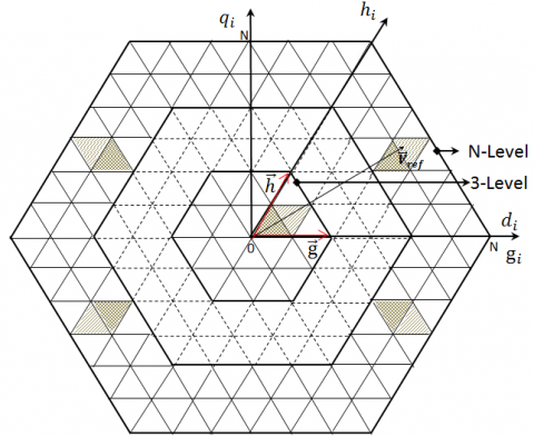
Figure 8 shows all of the vectors of commutation of the N levels converter, with the corresponding states of commutation in the new reference (g, h).
Figure 8. Commutation Vectors of the N levels converter in the (g, h) plan
In the field of the operating control in a diphase reference, as is the case in most modern control for the different machines, this can be carried out using a transformation by basic change (d, q)→(g, h) [25]. The result of the transformation matrix is as follows:
$\vec{V} \operatorname{ref}(g, h)=T_{1} \cdot \vec{V} \operatorname{ref}(d, q)$ (27)
$T_{1}=\frac{3}{2} \frac{N-1}{2} \cdot\left[\begin{array}{cc}1 & \frac{-1}{\sqrt{3}} \\ 0 & \frac{2}{\sqrt{3}}\end{array}\right]$ (28)
4.2 Detection of the nearest three vectors (NTV)
The switching vectors have integer coordinates. This is advantageous because the four vectors nearest to the reference vector can be simply identified; these vectors whose coordinates are combinations of the rounded values greater and lower than the number of the reference vector are calculated as follows:
$\overrightarrow{V_{u l}}=\left[\begin{array}{l}{\left[V_{r e f g}\right]} \\ {\left[V_{r e f h}\right]}\end{array}\right], \overrightarrow{V_{l u}}=\left[\begin{array}{l}\left.| V_{r e f g}\right\rfloor \\ {\left[V_{r e f h} |\right.}\end{array}\right]$
$\overrightarrow{V_{u u}}=\left[\begin{array}{l}{\left[V_{r e f g}\right]} \\ {\left[V_{r e f h}\right]}\end{array}\right], \overrightarrow{V_{l l}}=\left[\begin{array}{l}\left|V_{r e f g}\right| \\ \left|V_{r e f h}\right|\end{array}\right]$
with:
⌈Vref⌉: Indicates the upper rounded value of Vref;
⌊Vref⌋: Indicates the lower rounded value of Vref
The final points of the four nearest vectors form the equal parallelogram, which is divided into two equilateral triangles by the diagonal connecting the vectors Vul. These are always two of the NTV. The third nearest vector is one of the two remaining vectors existing on the same side of the diagonal; it is taken as a reference. For that reason, the closest third vector can be found by evaluating the sign of the expression:
Ð=$V_{\text {refg}}+V_{\text {refh}}-\left(V_{\text {ulg}}+V_{\text {ulh}}\right)$ (29)
If the variable Ð is positive, then the vector Vuu is the third nearest vector. That is, the vector Vll is the nearest third vector. This concludes the identification of NTV for N-level inverters. Figure 9 explains how to obtain the closest third vector.
Figure 9. Localization of two different cases of the position of reference vector of the same four nearest vectors
4.3 Calculation of the switching times of the switches
The best way to synthesize the voltage reference vector is to use the three nearest vectors
$\vec{V} \operatorname{ref}=d_{1} \vec{V} 1+d_{2} \vec{V} 2+d_{3} \vec{V} 3$ (30)
With the following additional constraint on the conduction times:
$d_{1}+d_{2}+d_{3}=1$ (31)
Once the TVP are identified, the switching times of the switches can be found by solving (32) and (33), with:
$\left\{\begin{array}{l}\vec{V}_{1}=\vec{V}_{u l} \\ \vec{V}_{2}=\vec{V}_{l u} \\ \vec{V}_{3}=\vec{V}_{l l}\end{array}\right.$ (32)
$\left\{\begin{array}{l}\vec{V}_{1}=\vec{V}_{u l} \\ \vec{V}_{2}=\vec{V}_{l u} \\ \vec{V}_{3}=\vec{V}_{u u}\end{array}\right.$ (33)
Since all switching vectors always have integer coordinates, the solutions are essentially the partial parts of the coordinates (Figure 10).
If $\vec{V}_{3}=\vec{V}_{l l}$ Then $\left\{\begin{array}{l}d_{u l}=V_{r e f g}-V_{l l g} \\ d_{l u}=V_{r e f h}-V_{l l h} \\ d_{l l}=1-d_{u l}-d_{l u}\end{array}\right.$ (34)
If $\vec{V}_{3}=\vec{V}_{u u}$ Then $\left\{\begin{aligned} d_{u l} &=-\left(V_{r e f h}-V_{u u h}\right) \\ d_{l u} &=-\left(V_{r e f g}-V_{u u g}\right) \\ d_{l l} &=1-d_{u l}-d_{l u} \end{aligned}\right.$ (35)
4.4 Algorithm of three-phase SVM, N level
The algorithm of three-phases SVM of N levels inverters is summarized in Figure 10.
Figure 10. Algorithm of three-phase SVM, N level
In this part, an indirect field oriented control (IFOC) induction machine drive by a conventional PI practical to the SPIM is presented. The IFOC technique is principally a predictive approach in that it approximates the angular position of the rotor flux vector by exploiting the model of the SPIM [35,37]. A commonly used IFOC technique uses the following equations to satisfy the condition for proper orientation. Geometrically speaking, we will say that the stator variables projected on the plane (d-q) are involved in the electromechanical conversion of energy. In contrast, the stator variables projected on the plane (x-y) are not involved in the electromechanical conversion of energy. This decoupling will simplify the analysis and control of the SPIM. Orienting the axis system (d-q) so that the axis d is in phase with the rotor flow (Figure 11), to obtain:
$\left\{\begin{array}{c}\varphi_{r d}=0 \\ \varphi_{r q}=\varphi_{r}\end{array}\right.$ (36)
Figure 11. The orientation of the rotor flow
The system of equations becomes:
$\left\{\begin{aligned} \varphi_{s d} &=L_{s}\left(1-\frac{M^{2}}{L_{s} L_{r}}\right) i_{s d}+\frac{M}{L_{r}} \varphi_{r} \\ \varphi_{s q} &=L_{s}\left(1-\frac{M^{2}}{L_{s} L_{r}}\right) i_{s q} \\ i_{r d} &=\frac{1}{L_{r}}\left(\varphi_{r}-M i_{s d}\right) \\ i_{r q} &=\frac{M}{L_{r}} i_{s q} \end{aligned}\right.$ (37)
$\left\{\begin{array}{l}V_{s d}=R_{s} i_{s d}+\sigma L_{s} \frac{d i_{s d}}{d t}-\omega_{s} \sigma L_{s} i_{s q} \\ V_{s q}=R_{s} i_{s q}+\sigma L_{s} \frac{d i_{s q}}{d t}+\omega_{s} \frac{M}{L_{r}} \varphi_{r}+\omega_{s} \sigma L_{s} i_{s d} \\ M i_{s d}=\varphi_{r d}+T_{r} \frac{d \varphi_{r d}}{d t} \\ \omega_{r}=\omega_{s}-\omega=\dot{\theta}=p \Omega=\frac{M}{T_{r}} \frac{i_{s q}}{\varphi_{r}}\end{array}\right.$ (38)
Then using PI regulator of the obtained linearized systems (38). A comprehensive speed regulation diagram of the SPIM by the IFOC presented on the Figure 12.
Figure 12. The control strategy of speed closed loop on six-phase
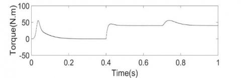
In this section, the validation of the dual SVM three-phase multilevel inverter to control an SPIM with IFOC is achieved. The SPIM parameters present in the Appendix. Figure 13 presents a speed response $\gamma=60^{\circ}$ represented with the application of a load torque, Cr=40N.m, at time t=0.4s, and reversing the direction of rotation at time 0.7s from 40rad/s to 60 rad/s, it can be observed that the machine speed follows the reference. When the load torque is applied, at the instant t = 0.4s, the speed is reduced, but it is re-established again without static error, and the torque magnitude increases 0Nm to 40Nm showed in Figure 14 and remain constant at 40Nm as shown. When the reference speed is changed during simulation, the actual speed is observed to follow the change in speed as is seen from Figure 13. At the instant of speed change (0.7s), a spike is observed in the torque waveform Figure 14 which is attributed to the sudden change of speed. The actual speed is observed to track the reference. So, it highlights the good performance of the proposed structure, and we obtain the same results for $\gamma=30^{\circ}, 0^{\circ}$ in the speed and the torque electromagnetic. At the instant t = 0.4 s where the load torque is applied, the speed is reduced, but it is re-established again without static error.
Figure 13. Simulation results of speed response of the SPIM with application of a load torque resistant, Cr=40N.m, at time t=0.4s
Figure 14. Electromagnetic torque for Cr=40N.m.
The stator current is shown in Figure 15 for $\gamma=60^{\circ}$. Initially, at the start, the current is observed to have a lot of ripples because of not using starting techniques. It can be seen that IFOC offered better dynamic performance for speed control and proved to be a better solution for variable speed drives.
Figure 15. Stator currents of the SPIM with application of a load torque resistant, Cr=40N.m
Figure 16 presents SPIM simulations results for displacement between stator winding ($\gamma=0^{\circ}, 30^{\circ}, 60^{\circ}$). The obtained six-stator currents similarly for $\gamma=0^{\circ}, 30^{\circ}, \text{and } 60^{\circ}$.
- Figure 16 (A) presents the current superposed two three-phase IM $\gamma=0^{\circ}$;
- Figure 16 (B) presents the current of asymmetrical six-phase IM for $\gamma=30^{\circ}$;
- Figure 16 (C) presents the current of symmetrical six-phase IM for $\gamma=60^{\circ}$.
Figure 16. Phase currents for (A) dual three-phase, for (B) asymmetrical six-phase IM, and (C) symmetrical six-phase IM
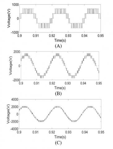
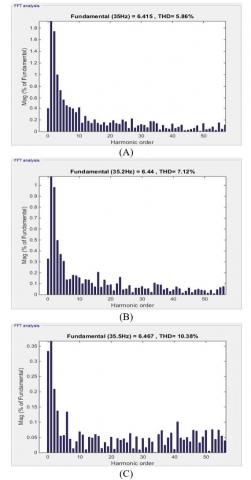
The results obtained using three configurations of the SPIM are presented in Figure 17
- Figure 17 (A) shows the output of the three levels inverter. The simulation results show the three levels of the output voltage. The THD is obtained as 10.38 % by FFT analysis in simulation and is shown in the figure 18 (A);
- Figure 17 (B) shows the output of the five levels inverter. The simulation results show the five levels of the output voltage. The THD is obtained as 7.12 % by FFT analysis in simulation and is shown in the figure 18 (B);
- Figure 17 (C) shows the output of the seven levels inverter. The simulation results show the seven levels of the output voltage. The THD is obtained as 5.86 % by FFT analysis in simulation and is shown in the figure 18 (C).
Figure 17. Phase voltage for (A) three-level, for (B)five-level, and (C) seven-level
We find that when increasing the number of levels, the tensions will be closer to the sinusoid
Figure 18. Percentage of the THD according to the angle $\gamma$ with different levels (3L, 5L, and 7L)
The results obtained using three configurations of the IM are presented in Figure 19 with $\gamma=30^{\circ}$
- Figure 19 (A) presents current for three levels;
- Figure 19 (B) presents current for five levels;
- Figure 19 (C) presents current for seven levels.
Figure 19. Phase currents for (A) three-level, for (B) five-level, and (C) seven-level for $\gamma=30^{\circ}$
Clearly, when the level number increases, the stator's currents become smooth and better. We find that when the number of levels increases, the stator currents become smoother. The following Table I summarizes the percentage of the THD according to the angle $\gamma$ with different levels (3L, 5L, and 7L). In fact, it is clearly observable in table 1 the THD% decreases gradually and progressively as the number of levels of the inverter increases. According to the results found there that when the level of the inverter voltage is N=3, N=5 and N =7 the output voltage approaches more and more perfect sinusoidal form. Best THD for $\gamma=30^{\circ}$ phase shift angle and level 7.
Table 1. Percentage of the THD according to angle $\gamma$ with different levels for SPIM
|
|
For $\gamma=0^{\circ}$ |
For $\gamma=30^{\circ}$ |
For $\gamma=60^{\circ}$ |
||||||
|
THD % |
3l |
5l |
7l |
3l |
5l |
7l |
3l |
5l |
7l |
|
10.38 |
7.12 |
5.86 |
10.35 |
7.10 |
5.82 |
10.36 |
7.11 |
5.83 |
|
This paper presents a new dual SVM algorithm for the six-phase multilevel inverter-SPIM. Where the six phase multilevel inverter has controlled as two three-phase multilevel inverter separately by the N-level SVM of the three-phase SDCS inverter. The two three-phase multilevel inverter diphase by γ=0°, γ=30° and γ=60°, according to the type of the six phases machine with placed windings; two three-phase induction machine, asymmetric six phase, symmetrical six-phase IM respectively. This control strategy of the N-level inverters SDCS is general, applicable to any number of levels converter, where the number of steps involved in computation is always the same despite the area of the reference voltage vector. In addition to that, the efficiency and the ease of implementation of this algorithm makes it well suited for simulation on digital computers, and can become a very useful device in assist investigation of the properties of multilevel power converters. The main advantage of phase shift γ is to show that the dual SVM is general regardless of the phase shift γ. It has been shown by simulation that the stator current harmonic loss and output torque ripple are reduced. The studied SPIM multilevel inverter is suited for applications requiring high power synchronous motor drives.
Machine parameters: Rated Power: Pn=5,5 kW, Rated voltage: Vn=220 V, Rated current: In=6 A, Rated speed: Nn=1000 rpm, Number of poles: P=6, Stator resistance: Rs=2.03 Ω, Rotor resistance: Rr=3 Ω, Stator inductance: Ls=0.2147 H, Rotor inductance: Lr=0.2147 H, Mutual inductance: M=0.2 H, Moment of inertia: J=0.06 kg.m2.
Acronyms
SVM: Space Vector Modulation
SPIM: Six Phase Induction Machine
IFOC: Indirect Field Oriented Control
VSI: Voltage-Source Inverter
PWM: Pulse Width Modulation
SDCS: Separate Direct Current Source
NTV: Nearest Three Vectors
VSD: Vector Space Decomposition
[1] Khadar, S., Kouzou, A., Hafaifa, A., Iqbal, A. (2019). Investigation on SVM-Backstepping sensor-less control of five-phase open-end winding induction motor based on model reference adaptive system and parameter estimation. Engineering Science and Technology, an International Journal, 22(4): 1013-1026. https://doi.org/10.1016/j.jestch.2019.02.008
[2] Khadar, S., Kouzou, A., Rezzaoui, M.M., Hafaifa, A. (2019). Sensor-less control technique of open-end winding five phase induction motor under partial stator winding short-circuit. Periodica Polytechnica Electrical Engineering and Computer Science, 64(1): 2-19. https://doi.org/10.3311/PPee.14306
[3] Gan, C., Sun, Q., Wu, J., Shi, C.W, Hu, Y. (2019). A universal two-sensor current detection scheme for current control of multi-phase switched reluctance motors with multi-phase excitation. IEEE Trans.on Power Electronics, 34(2): 1526-1539. https://doi.org/10.1109/TPEL.2018.2830308
[4] Rahali1, H., Zeghlache, S., Benalia, L., Layadi, N. (2018). Sliding mode control based on backstepping approach for a double star induction motor (DSIM). Advances in Modelling and Analysis C, 73(4): 150-157. https://doi.org/10.18280/ama_c.730404
[5] Kumar, P.R., Karthik, R.S., Gopakumar, K., Leon, J.I., Franquelo, L.G. (2015). Seventeen-level inverter formed by cascading flying capacitor and floating capacitor H-bridges. IEEE Trans. Power Electron, 30(7): 3471-3478. https://doi.org/10.1109/TPEL.2014.2342882
[6] Belkamell, H., Mekhilef, S., Masaoud, A., Naeim, M.A. (2013). Novel three phase asymmetrical cascaded multilevel voltage source inverter. IET Power Electron, 6(8): 1696-1706. https://doi.org/10.1049/iet-pel.2012.0508
[7] Layadi, N., Zeghlache, S., Benslimane, T., Berrabah, F. (2017). Comparative analysis between the rotor flux oriented control and backstepping control of a double star induction machine (DSIM) under open-phase fault. Advances in Modelling and Analysis C, 72(4): 292-311.
[8] Nair, R., Rahul, A., Gopakumar, S.K., Leopoldo, G.M Franquelo, Fellow, Williamson, S., Member, S. (2017). Stacked multilevel inverter fed six phase induction motor with reduced DC link and lower voltage devices. IEEE International Conference on Industrial Technology (ICIT), 25 March 2017, Toronto, ON, Canada. https://doi.org/10.1109/ICIT.2017.7913254
[9] Odeh, C.I. (2015). Sinusoidal pulse-width modulated three-phase multi-level inverter topology. Electric Power Components and Systems, 43(1): 1-9. https://doi.org/10.1080/15325008.2014.963260
[10] Che, H.S., Duran, M.J., Levi, E., Jones, M., Hew, W.P., Ahim, N.A. (2014). Post fault operation of an asymmetrical six-phase induction machine with single and two isolated neutral points. IEEE Transactions on Power Electronics, 29(10): 5406-5416. https://doi.org/10.1109/TPEL.2013.2293195
[11] Grandi, G., Tani, A., Vikumar, P.S., Ostojic, D. (2010). Multi-phase multi-level ac motor drive based on four three-phase two-level inverters. Power Electronics Electrical Drives Automation and Motion(SPEEDAM), International Symposium on, June 2010, Pisa, Italy. https://doi.org/10.1109/SPEEDAM.2010.5545091
[12] Jones, M., Patkar, F., Levi, E. (2013). Carrier-based pulse-width modulation techniques for asymmetrical six-phase open-end winding drives. Electric Power Applications, 7(6): 441-452. https://doi.org/10.1049/iet-epa.2012.0372
[13] Odeh, C.I., Obe, S.E., Ojo, O. (2016). Topology for cascaded multilevel inverter. IET Power Electronics, 9(5): 921-929. https://doi.org/10.1049/iet-pel.2015.0375
[14] Duran, M.J., Barrero, F. (2016). Recent advances in the design, model ING, and control of multi-phase machines - Part II. IEEE Transactions on Industrial Electronics, 63(1): 459-468. https://doi.org/10.1109/TIE.2015.2448211
[15] Levi, E., Barrero, F., Duran, M.J. (2016). Multi-phase machines and drives-Revisited. IEEE Transactions on Industrial Electronics, 63(1): 429-432. https://doi.org/10.1109/TIE.2015.2493510
[16] Li, F., Hua, W., Tong, M., Zhao, G., Cheng, M. (2015). Nine-phase flux switching permanent magnet brushless machine for low-speed and high torque applications. IEEE Transactions on Magnetics, 51(3): 1-4. https://doi.org/10.1109/TMAG.2014.2364716
[17] Levi, E. (2016). Advances in converter control and innovative exploitation of additional degrees of freedom for multi-phase machines. IEEE Transactions on Industrial Electronics, 63(1): 433-448. https://doi.org/10.1109/TIE.2015.2434999
[18] Babu, N., Agarwal, P. (2018). Nearest and non-nearest three vector modulations of NPCI using two-level space vector diagram-A novel approach. IEEE Transactions on Industry Applications, 54(3): 2400-2415. https://doi.org/10.1109/TIA.2017.2787629
[19] Karasani, R.R., Borghate, V.B., Meshram, P.M., Surya wanshi, H.M., Sabyasachi, S. (2017). A three-phase hybrid cascaded modular multilevel inverter for renewable energy environment. IEEE Transactions on Power Electronics, 32(2): 1070-1087. https://doi.org/10.1109/TPEL.2016.2542519
[20] Kalaiselvi, J., Srinivas, S. (2015). Bearing currents and shaft voltage reduction in dual-inverter-fed open-end winding induction motor with reduced cmv PWM methods. IEEE Transactions on Industrial Electronics, 62(1): 144-152. https://doi.org/10.1109/TIE.2014.2336614
[21] Marouani, K., Nounou, K., Benbouzid, M.E.H., Tabbache, B. (2016). Investigation of energy efficiency improvement in an electrical drive system based on multi-winding machines. Electrical Engineering, 100: 205-216. https://doi.org/10.1007/s00202-016-0493
[22] Lopez, I., Ceballos, S., Pou, J., Zaragoza, J., Andreu, J., Kortabarria, I., Agelidis, V.G. (2016). Modulation strategy for multi-phase neutral-point clamped converters. IEEE Transactions Power. Electron, 31(2): 928-941. https://doi.org/10.1109/TPEL.2015.2416911
[23] Nair, V., Rahul, A., Kaarthik, R., Kshirsagar, A., Gopakumar, K. (2016). Generation of higher number of voltage levels by stacking inverters of lower multilevel structures with low voltage devices for drives. IEEE Transactions on Power Electronics, 32(1): 52-59. https://doi.org/10.1109/TPEL.2016.2528286
[24] Leon, J.I., Kouro, S., Franquelo, L.G., Rodriguez, J., Wu, B. (2016). The essential role and the continuous evolution of modulation techniques for voltage-source inverters in the past, present, and future power electronics. IEEE Transactions Ind. Electron, 63(5): 2688-2701. https://doi.org/10.1109/TIE.2016.2519321
[25] Thamizharasan, S., Baskaran, J., Ramkumar, S. (2015). A new cascaded multilevel inverter topology with voltage sources arranged in matrix structure. Journal of Electrical Engineering and Technology, 10(4); 1552-1557. https://doi.org/10.5370/JEET.2015.10.4.1552
[26] Kong, W., Huang, J., Kang, M., Li, B., Zhao, L.H. (2014). Fault-tolerant control of five-phase induction motor under single-phase open. Journal of Electrical Engineering and Technology, 9(3): 899-907. https://doi.org/10.5370/JEET.2014.9.3.899
[27] Costa, N., Melo, F., Freitas, L., Coelho, E., Freitas, L.C.G. (2013). Multilevel inverter based on cascaded association of Buck EIE inverters. IET Power Electron, 6(6): 1165-1174. https://doi.org/10.1049/iet-pel.2012.0684
[28] Bduallah, A.A., Dordevic, O., Jones, M. (2017). Multidirectional power flow control among double winding six-phase induction machine winding sets. 43rd Annual Conference of the IEEE Industrial Electronics Society, 29 Oct.-1 Nov. 2017, Beijing, China. https://doi.org/10.1109/IECON.2017.8217403
[29] González-Prieto, I., Duran, M.J., Barrero, F.J. (2017). Fault-tolerant control of six-phase induction motor drives with variable current injection. IEEE Transactions on Power Electronics, 32(10): 7894-7903. https://doi.org/10.1109/TPEL.2016.2639070
[30] Nair, R.V., Rahul, A.S., Pramanick, S., Gopakumar, K., Franquelo, L.G. (2017). Novel symmetric six-phase induction motor drive using stacked multilevel inverters with a single DC link and neutral point voltage balancing. IEEE Transactions on Industrial Electronics, 64(4): 2663-2670. https://doi.org/10.1109/TIE.2016.2637884
[31] Holakooie, M.H., Ojaghi, M., Taheri, A. (2018). Direct torque control of six-phase induction motor with a novel MRAS-based stator resistance estimator. IEEE Transactions on Industrial Electronics, 65(10): 7685-7696. https://doi.org/10.1109/TIE.2018.2807410
[32] Pandit, K.J., Aware, M.V., Nemade, R., Levi, E. (2017). Direct torque control scheme for a six-phase induction motor with reduced torque ripple. IEEE Transactions on Power Electronics, 32(9): 7118-7129. https://doi.org/10.1109/TPEL.2016.2624149
[33] Felipe, V., Melo, M.B., Jacobina, C.B., Rocha, N. (2018). Fault tolerance performance of dual-inverter based six-phase drive system under single-, two-, and three-phase open-circuit fault Operation. IET Power Electron, 11(1): 212-220. https://doi.org/10.1049/iet-pel.2016.0724
[34] Bouhali1, O., Francois, B., Rizoug, N. (2014). Equivalent matrix structure modelling and control of a three-phase flying capacitor multilevel inverter. ET Power Electron, 7(7): 1787–1796. https://doi.org/10.1049/iet-pel.2013.0414
[35] Hellali, L., Belhamdi, S., Loutfi, B., Hassen, R. (2018). Direct torque control of doubly star induction machine fed by voltage source inverter using type-2 fuzzy logic speed controller. Advances in Modelling and Analysis C, 73(4): 137-149.
[36] Lekhchine, S., Bahib, T., Soufi, Y. (2014). Indirect rotor field oriented control based on fuzzy logic controlled double star induction machine. Electr Power Energy Sys, 57: 206–211. https://doi.org/10.1016/j.ijepes.2013.11.053
[37] Belhamdi, S., Goléa, A. (2015). Direct Torque Control for Induction Motor with broken barsusing Fuzzy Logic Type-2. Advances in Modelling and Analysis C, 70(1): 15-28.