OPEN ACCESS
The changed power system regulations, liberalization in distribution market and enhanced use of power electronics based equipment has raised the concerns about power quality (PQ). Though, the responsibility of PQ deterioration is shared by both utility and its consumers; the most influencing factor to the poor PQ is the consumer’s load. The estimation of individual consumers’ responsibility is a herculean task for the utilities. In this paper, a technique based on S-transform is proposed for the identification of the load responsible for specific type of PQ disturbance and the estimation of its responsibility in causing PQ deterioration at the point of common coupling (PCC). The main objective of this work is to fill the void in the PQ study by including utility’s perspective. This paper presents a simple approach to identify the share of consumer’s load that causes the PQ deterioration at the PCC. The proposed method is validated by PCC signals acquired by both MATLAB simulations and by using laboratory experimental setup.
identification, estimation, power quality, signal processing, power distribution
The advent of smart grid, changed power system regulations, liberalized distribution market and increased use of nonlinear devices in today’s distribution system has increased the concerns about power quality (PQ). Partial or complete failures of equipment and loss of important data are amongst the major detrimental consequences of poor PQ. Both, utility and its consumers, are equally affected by the poor PQ. At the same time, both are responsible for the PQ deterioration too.
The regular operations of the utilities such as, load switching, power factor correction bank switching and fault clearing can cause PQ deterioration. However, these operations are essential to maintain continuous supply to the consumers. On the other hand, the consumer loads are the major contributor towards PQ deterioration. The consumers are expected to make sure that their load does not affect the utility supply and consequently the other consumers connected to the same Point of Common Coupling (PCC) [1]. In fact, the problem of locating the specific consumer load causing the PQ deterioration is more difficult task for the utility [2].
Most of the studies are concentrated towards the consumer’s point of view. However, the utility’s perspective is equally important. For this purpose, IEEE 519-1993 standards recommends the use of PQ indices such as; total harmonic distortion (THD) and total demand distortion (TDD), for locating the consumer load, responsible for the deterioration of PQ at the PCC [3]. However, these indices are restricted to stationary PQ disturbances only, while non-stationary disturbances such as; voltage sag, swell, interruptions, impulsive, and oscillatory transients are not addressed. Moreover, THD and TDD are based on Fourier transform (FT), which is insufficient for the analysis of non-stationary disturbances [4]. The non-stationary disturbances are broadly defined in terms of their spectral content, magnitudes and durations by IEEE 1159-2009 [5].
The issue of identifying the specific disturbance source and the measurement of their individual responsibility is scantly addressed in the literature. In [6], a method to quantify the customer and utility responsibilities for limit violations caused by either harmonic source changes or harmonic impedance changes is proposed. Discrete Wavelet Transform (DWT) based harmonic source detection is discussed in [7]. Literatures [8-11] report important contribution towards the stationary harmonic disturbance estimation. While, these methods account stationary harmonics; non-stationary disturbances are not addressed. In [12] an ATP simulated distribution system is used for finding the direction of the disturbance source by examining the energy flow and peak instantaneous power for both capacitors energizing and voltage sag disturbances. In [13], a method based on the branch current is presented for tracking sag and capacitor switching transients. Some important contributions towards the detection of the voltage sag sources are reported in [14-16]. These approaches do address non-stationary sag and capacitive transients, but do not account harmonics at the same time.
Signal processing techniques based on time-frequency distribution are well utilized for the analysis of the non-stationary PQ issues to overcome these difficulties. Several signal processing techniques have been used to define PQ indices to quantify non-stationary disturbances [17-25]. Short time Fourier transform (STFT) based power quality quantification is suggested in [17]. STFT based methods are always a compromise between time and frequency resolution caused by fixed window width. In [18], a DWT based reformulated PQ indices from the conventional PQ indices are presented. However, the approach is limited to stationary disturbances only. PQ indices based on wavelet packet transform are defined in [19-20]. PQ indices based on Cohen’s class [21] and based on S-transform [22] are also developed. Time-frequency distribution based methods have been employed for the identification and classification of non-stationary PQ disturbances in [23-25].
PQ index based on S-transform; instantaneous form factor, IFF(τ) defined by the author, is utilized in this paper to analyze a test distribution system [26]. Three consumer loads causing harmonics, voltage sag and oscillatory transients are considered to be supplied by the same PCC. The voltage and current signals are acquired at the PCC for all the possible load combinations and analyzed for the responsibility estimation purpose. The PQ disturbance sources while acting together would cause simultaneous PQ disturbance, which is captured by index IFF(τ). Then the same PQ disturbance sources, while acting individually on the PCC the IFF(τ) index is computed. Based on the comparison of these data, the proposed method estimates the responsibility of individual disturbance source.
The rest of the paper is organized as follows: Section 2 describes the model distribution system used for the acquisition of the voltage and current signals for the validation. Section 3 briefly covers the S-transform and the mathematical computation of the index IFF(τ). The complete flow chart of the proposed approach is explained in Section 4 including the results and discussions. Finally, the conclusions are made in section 5.
The acquisition of PQ signal data plays an important role in defining and establishing the appropriateness of the methodology. From the utility point of view, the PCC is the place where the PQ measurements are generally made. PCC is the point where the correct judgment regarding the health of the distribution system can be made, as the nature of the consumer loads connected on it are the major contributor toward the deteriorated PQ.
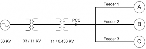
The one-line diagram of the model distribution system considered for the acquisition of the signal database is shown in Figure 1. Three consumers (referred as the PQ disturbance sources) producing harmonics (consumer A), voltage sag (consumer B) and oscillatory transients (consumer C) are considered to be connected to the same PCC. The PQ disturbance sources causing different types of disturbances are considered as:
Source A: Produces harmonics at the PCC voltage signal having THD variation of 4.82 % to 26.07 %.
Source B: Produces voltage sag at the PCC voltage signal having 2 cycle duration to 5 cycle sag duration.
Source C: Produces oscillatory transient at the PCC voltage signal having 3.8 kHz to 8 kHz natural frequency.
Figure 1. Single line representation of a typical distribution system
The impact of each disturbance type can be controlled in four steps as shown in Table 1. Further, these sources are considered to be acting on the PCC in all ten possible ways as shown in Table 2; e.g. Case-I in Table 2 represents the following disturbance source combination: Source-A producing 13.01 % THD, Source-B injecting 8 kHz oscillatory transient and voltage sag variations of 2 cycle caused by Source-C. For each case of Table 2, PCC voltage and feeder current signals are acquired for the analysis.
Table 1. Variation in different disturbances considered for the analysis
|
Source A |
Source B |
Source C |
|
% THD |
Duration of Sag (cycle) |
Frequency (kHz) |
|
4.82 |
2 |
3.5 |
|
6.12 |
3 |
4.8 |
|
13.01 |
4 |
6.0 |
|
26.07 |
5 |
8.0 |
Table 2. Different cases of PQ disturbance sources considered for the analysis
|
Cases |
A % THD |
B Duration of Sag (cycle) |
C Frequency (kHz) |
|
I |
13.01 |
2 |
8.0 |
|
II |
13.01 |
3 |
8.0 |
|
III |
13.01 |
4 |
8.0 |
|
IV |
13.01 |
5 |
8.0 |
|
V |
13.01 |
4 |
3.5 |
|
VI |
13.01 |
4 |
4.8 |
|
VII |
13.01 |
4 |
6.0 |
|
VIII |
6.12 |
4 |
8.0 |
|
IX |
4.82 |
4 |
8.0 |
|
X |
26.07 |
4 |
8.0 |
Table 3. Combinations disturbance sources
|
Sr. No |
Disturbance Source Combinations |
Type of Disturbance present in the acquired PQ signals |
|
1 |
A |
Harmonics only(A) |
|
2 |
B |
Sag only(B) |
|
3 |
C |
Oscillatory(C) |
|
4 |
AB |
Harmonics(A) + Sag(B) |
|
5 |
BC |
Sag(B) + Oscillatory(C) |
|
6 |
CA |
Oscillatory(C) + Harmonics(A) |
|
7 |
ABC |
Harmonics(A) + Sag(B) + Oscillatory(C) |
Further for each case of Table 2, the disturbance sources are combined in different combinations as depicted in Table 3; i.e. any one source at a time (A, B ,C); any two sources at a time(AB, BC, CA) and all three sources connected to the PCC at a time (ABC).
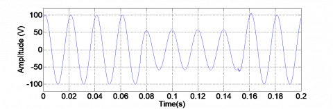
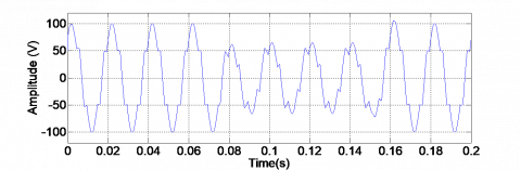
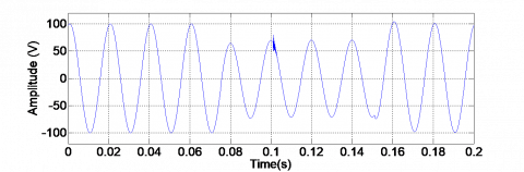
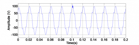
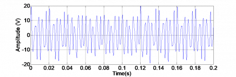
The typical PCC voltage signals acquired for case III of Table 2 are illustrated in Figure 2 to 4. Figure 2 shows the acquired voltage signals, when only one source is fed by the PCC at a time. Figures 3(a) to 3(c) show the voltage signals when two sources are simultaneously fed by the PCC and Figure 4 shows the voltage signal when all three sources are simultaneously fed by the PCC. These exercises give sufficient signals to analyze the effect of specific kind on disturbance on the PCC voltage signal. All the acquired signals are normalized at 100 magnitude peak to peak.
The distribution system is simulated using MATLAB. The voltage and current signals are acquired at the PCC and analyzed by computing the index; instantaneous form factor, IFF(τ). Throughout the paper, the index IFF(τ) is indicated as IFFV(τ) and IFFI(τ) when it is computed for the voltage and current signals respectively.
(a) Harmonics (A)
(b) Voltage sag (B)
(c) Oscillatory transient (C)
Figure 2. PCC voltage signals while PQ disturbance sources are connected alone
(a) Harmonics and sag (AB)
(b) Sag and oscillatory (BC)
(c) Oscillatory and harmonics (CA)
Figure 3. PCC voltage signals when two PQ disturbance sources are fed by the PCC simultaneously
Figure 4. PCC voltage signal when all three PQ disturbance sources are simultaneously fed by the PCC (ABC)
quired from PCC is addressed by utilizing an S-transform based index, instantaneous form factor (IFF(τ)) [26] in this work.
STFT gives a compromised time-frequency resolution caused by a fixed window width [17]. Continuous wavelet transform (CWT) solves this issue to a great extent. S-transform can be defined as a more refined version of CWT with a phase correction Gaussian window applied to it [27].
The S-transform of a signal x(t) can be mathematically expressed as,
$S(\tau ,f)=\frac{|f|}{\sqrt{2\pi }}\int\limits_{-\infty }^{+\infty }{x(t){{e}^{-\frac{{{(t-\tau )}^{2}}{{f}^{2}}}{2}}}}{{e}^{-2j\pi ft}}dt$ (1)
Hence in the case of S-transform, window width is inversely proportional to the frequency. It can be seen from (1) that, in the S-transform; the time localizing Gaussian is translated while the oscillatory exponential kernel remains stationary. By not translating the oscillatory exponential kernel, the S-transform localizes the real and the imaginary components of the spectrum independently, localizing the phase spectrum as well as the amplitude spectrum, and is thus directly invertible into the Fourier Transform Spectrum [27]. This makes S-transform more suitable for the analysis of the PQ disturbances.
The instantaneous form factor IFF(τ) used in this paper is mathematically defined by the author as [26];
$IFF(\tau )=\frac{\sqrt{\sum\limits_{{{f}_{\min }}}^{{{f}_{\max }}}{{{({{S}_{D}}(\tau ,f))}^{2}}}}}{\frac{1}{N}\sum\limits_{{{f}_{\min }}}^{{{f}_{\max }}}{|{{S}_{P}}(\tau ,f)|}}\,\ldots \ldots \forall \tau =0\quad to\quad N$ (2)
SD(τ,f) is the S-transform matrix of the separated disturbance signal and SP(τ,f) is the S-transform matrix for the estimated pure signal. Further the average and the peak values of IFF(τ) are also computed in order to have better understanding.
The acquired signal at the PCC carry the cumulative effects of all three PQ disturbance sources. Thus by analyzing these signals with appropriate mathematical indicator can certainly fetch information from it. The proposed approach is based on this notion.
The signals at PCC are analyzed with IFF(τ) and compared with the established PQ index, THD, to verify its usefulness for the analysis of the PQ at first. The results of the comparison are discussed in 4.1. The complete flow chart of the proposed approach for the identification and responsibility estimation is shown in Figure 5. The use of index IFF(τ) for the identification and responsibility quantification are further discussed in sections 4.2 and 4.3 respectively. Finally, in section 4.4 the proposed technique is applied to the real signals acquired by the laboratory PCC.
4.1 Comparison Between IFF(τ) and THD
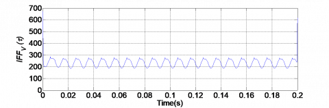
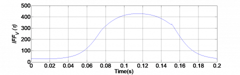
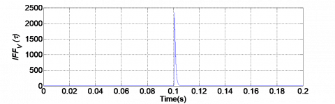
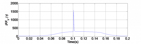
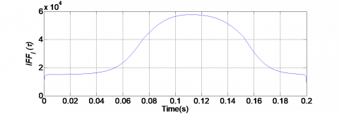
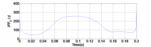
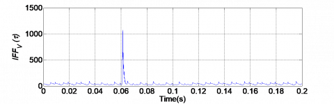
The IFF(τ) and THDs are calculated for all the acquired PCC voltage signals for all the cases and combinations shown in Tables 1, 2 and 3. Figure 6(a) to 6(c) show IFFV(τ) for the PCC voltage signals shown in Figure 2(a) to 2(c) respectively; i.e. when single PQ disturbance source is fed by the PCC. It can be observed here that for the stationary harmonics, the IFFV(τ) plot shows peaks distributed throughout the signal. The IFFV(τ) plot of voltage sag shows increased magnitude at the time of the disturbance and for the oscillatory transient, the IFFV(τ) plot shows a single peak at the time of disturbance. Thus IFFV(τ) plots of individual disturbances shows its usefulness in identifying the effect of corresponding type of source on the PCC.
Figure 5. Flow chart of the proposed technique for the identification of PQ disturbance sources and the quantification of their responsibility in PQ deterioration at PCC
(a) Harmonics (A)
(b) Sag (B)
(c) Oscillatory (C)
Figure 6. IFFV(τ) plot of PCC voltage when one PQ disturbance source is connected at a time on the PCC
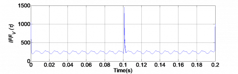
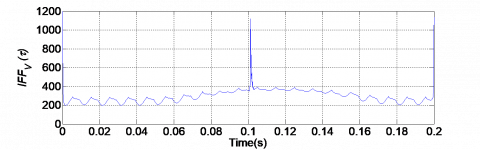
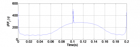
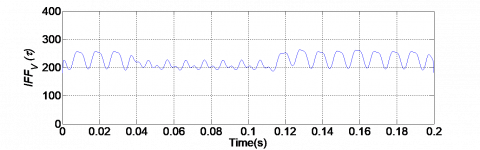
Figure 7(a) to 7(c) show IFFV(τ) for the PCC voltage signals of Figure 3(a) to 3(c) respectively when any two sources are fed simultaneously by the PCC. The plots clearly show the simultaneous effects of the two respective disturbances. Similarly, when all three PQ disturbance sources are fed by the same PCC, the PCC voltage signal analyzed by IFFV(τ) show the combined effects of all three as depicted in Figure 8. Thus, the index IFFV(τ) show its effectiveness in analyzing both stationary and non-stationary PQ disturbances.
The THDs of the acquired signals are calculated and listed in Table 4. The IFFV(τ) being a time dependent entity, the peak and average values of the IFFV(τ) are calculated and tabulated in Tables 5 and Table 6 respectively.
It can be observed in Table 4 that THD values show a small variation, even when the sag and oscillatory transient producing sources are connected to the PCC. As expected, THD is dominated by the effect of harmonic source (i.e. source A) while the other disturbances are not influenced in its value. e.g. in cases I to VII whenever source A is present, the value of THD is near to the value 13.01 %, which is actually caused by source A acting alone. The values of THDs fail to signify the effect of voltage sag and oscillatory transients.
(a) Harmonic and sag (AB)
(b) Sag and oscillatory (BC)
(c) Oscillatory and harmonics (CA)
Figure 7. IFFV(τ) plot of PCC voltage when two PQ disturbance sources are connected at a time on the PCC
Table 4. %THD calculated for different disturbance cases and combinations
|
Case Comb. |
I |
II |
III |
IV |
V |
VI |
VII |
|
ABC |
13.55 |
13.67 |
13.88 |
14.17 |
13.97 |
13.92 |
13.90 |
|
A |
13.01 |
13.01 |
13.01 |
13.01 |
13.01 |
13.01 |
13.01 |
|
B |
1.03 |
1.51 |
1.27 |
1.40 |
1.27 |
1.27 |
1.27 |
|
C |
0.42 |
0.42 |
0.42 |
0.42 |
0.63 |
0.53 |
0.47 |
|
AB |
12.88 |
13.01 |
13.31 |
13.81 |
13.31 |
13.31 |
13.31 |
|
BC |
0.91 |
0.91 |
0.99 |
1.05 |
1.05 |
1.02 |
1.00 |
|
CA |
13.25 |
13.25 |
13.25 |
13.25 |
13.58 |
13.55 |
13.53 |
Table 5. The peak values of IFFV(τ) for different disturbance cases and combinations
|
Case Comb. |
I |
II |
III |
IV |
V |
VI |
VII |
|
ABC |
1455.50 |
1058.39 |
1196.54 |
1124.01 |
1884.35 |
1792.01 |
1616.02 |
|
A |
671.42 |
671.42 |
671.42 |
671.42 |
671.42 |
671.42 |
671.42 |
|
B |
376.43 |
418.75 |
428.72 |
433.70 |
428.72 |
428.72 |
428.72 |
|
C |
2350.84 |
2350.84 |
2350.84 |
2350.84 |
2922.87 |
2961.34 |
2904.35 |
|
AB |
674.91 |
674.83 |
675.22 |
349.46 |
675.22 |
675.22 |
675.22 |
|
BC |
2354.61 |
1469.51 |
1594.24 |
1603.51 |
1950.88 |
1977.09 |
1940.37 |
|
CA |
1454.03 |
1454.03 |
1454.03 |
1454.03 |
2532.83 |
2404.79 |
2156.99 |
Table 6. The average values of IFFV(τ) for different disturbance cases and combinations
|
Case Comb. |
I |
II |
III |
IV |
V |
VI |
VII |
|
ABC |
271.97 |
282.69 |
295.52 |
308.13 |
297.39 |
296.43 |
295.73 |
|
A |
234.37 |
234.37 |
234.37 |
234.37 |
234.37 |
234.37 |
234.37 |
|
B |
127.75 |
167.51 |
207.14 |
248.47 |
207.14 |
207.14 |
207.14 |
|
C |
15.50 |
15.50 |
15.50 |
15.50 |
14.31 |
12.49 |
12.06 |
|
AB |
278.32 |
300.43 |
322.56 |
280.89 |
322.56 |
322.56 |
322.56 |
|
BC |
99.26 |
120.64 |
147.49 |
174.23 |
146.45 |
146.23 |
146.25 |
|
CA |
247.44 |
247.44 |
247.44 |
247.44 |
250.39 |
248.61 |
247.46 |
On the other end, IFFV(τ) show corresponding variation in peak and average values depending the type of sources producing disturbances are connected with the PCC. The peak values of IFFV(τ) are shown in Table 5. The values show that the oscillatory transients as they are related with the higher frequency content show higher peak values. Thus, whenever they accompany harmonics and/or the voltage sag they tend to dominate the peak value of IFFV(τ). The peak values are not affected much for the variations in sag durations in cases I to IV, which is because in these cases the magnitude of sag is not varied and only the durations are varied. This fact is very well depicted by the average value of IFFV(τ) as shown in Table VI, which show a corresponding increase with the increase in the sag duration from 2 cycle to 5 cycles in the cases I to IV. Harmonics being stationary disturbances, both average and peak values of IFF(τ) are affected by them as can be observed in Tables 5 and 6.
4.2 Identification of PQ disturbance sources
As explained in the previous sub-section, IFFV(τ) of the PCC voltage signal, indicates the cumulative effects of all the PQ disturbance sources which are connected to the PCC. However, in order to identify the source of specific PQ disturbance the acquired signals have to be analyzed further.
To identify the specific source responsible for particular PQ disturbance, among the sources connected to the PCC, the current signals of the individual feeders supplying to the sources are analyzed with IFFI(τ) as shown in Figure 5. Two cases are considered; in the first case sources A and B are connected to PCC and in the second case sources A, B and C are connected to PCC. In each case the PCC voltage signal and the individual feeder current signals are acquired and analyzed.
For the first case, when sources A and B are fed by the PCC, the PCC voltage are shown in Figure 3(a) and corresponding IFFV(τ) is shown in Figure 7(a). The currents in the feeders supplying A and B are also acquired and their IFFI(τ) are computed. Figure 9(a) and 9(b) show IFFI(τ) plots for current signals of source A and B, respectively. It can be observed from Figure 9(a) and 9(b) that, on IFFI(τ) the effect of the corresponding disturbance only dominates, while the effect of the other disturbance is minimized; e.g. in IFFI(τ) plot of Figure 9(a), the effect of harmonics is prominent while the effect of sag is minimum. Similarly, in IFFI(τ) plot of Figure 9(b), the effects of sag are prominent while the effects of harmonics are negligible.
In the second case, all three PQ disturbance sources A, B and C are fed simultaneously by the PCC. The corresponding plots of IFFV(τ) for PCC voltage signal and IFFI(τ) of the feeder current signals are shown in Figure 8 and Figure 10. Again, note that the corresponding PQ disturbance only dominates in the IFFI(τ) plots of current signals. Although, in Figure 10(c) the plot looks like having oscillatory transient and sag together, the effect of oscillatory is still prominent.
(a) Current of the feeder that supplies source A
(b) Current in the feeder that supplies source B
Figure 9. IFFI(τ) of the current signals acquired at PCC when two PQ disturbance sources are fed
(a) Current of the feeder that supplies source A
(b) Current in the feeder that supplies source B
(c) Current in the feeder that supplies source C
Figure 10. IFFI(τ) of the current signals acquired at PCC when three PQ disturbance sources are fed
Thus, by observing the IFFV(τ) plot of the PCC voltage and at the same time the IFFI(τ) plots of the respective current signals of the feeders, it is possible to pinpoint the sources which are responsible for respective disturbance at the PCC. This method can be further improved by using the automatic classification algorithms such as [23-25].
4.3 Quantification of the responsibility of the individual PQ disturbance source
The PCC voltage signal and its corresponding IFFV(τ), similar to the signals shown in Figure 4 and Figure 8, can be used to identify PQ disturbance sources (i.e. A, B and C in this work). Once the type of disturbance sources is identified, it is essential to somehow isolate the effects of individual source to estimate individual disturbance source’s responsibility to PQ deterioration at the PCC. For this purpose, the proposed approach relies on filters and IFFV(τ).
To isolate the effect of an individual source, the acquired PCC voltage signals are processed through three IIR filters; low pass filter (LPF), high pass filter (HPF) and a band-pass filter (BPF), as shown Figure 5. The frequency content of voltage sag is mainly composed of a fundamental frequency [11]. Thus, to isolate voltage sag signals, LPF is designed with 100 Hz cut-off frequency. Usually, the harmonics are caused by three phase rectifier which has prominent harmonics in the order of 5th and 7th (i.e. 250 Hz and 350 Hz). Thus, to isolate harmonics, BPF is designed with lower and higher cut-off frequencies of 100 Hz and 1000 Hz, respectively. Note that voltage signals still can have higher order harmonics. However, the effects of higher order harmonics are negligible. To extract oscillatory transients, the HPF is designed with 1000 Hz cut-off frequency.
(a) Band pass filter output capturing harmonic signal
(b) Low pass filter output capturing voltage sag
(c) High pass filter output capturing oscillatory transient
Figure 11. Filtered signals of PCC voltage signal of Figure 4
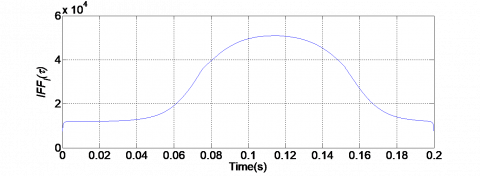
Once the PCC voltage signal is filtered, it is easier to evaluate IFFV(τ) of each filtered signal to quantify the responsibility of the corresponding source. The filtered PCC voltage signals and their corresponding IFFV(τ) are shown in Figure 11(a)-(c) and Figure 12(a)-(c), for harmonics (Source A), sag (Source B) and oscillatory transient (Source C), respectively.
Further, for these filtered signals the peak and average values of IFFV(τ) are calculated and summarized in Tables 7 and 8. The peak and average value of IFFV(τ) can be used to quantify each source’s contribution toward total PQ deterioration. For example, for Case-I the peak value of IFFV(τ) for Source-C (Oscillatory transient) in Table 7 is quite high compared to the other sources while its average value in Table 8 is comparatively lower. This is in agreement with the results shown in Figure 6.
(a) Harmonic signal
(b) Voltage sag signal
(c) Oscillatory transient signal
Figure 12. IFFV(τ) plots for processed PCC voltage signals
Note that, the proposed approach does not require any disconnection; it relies on the measured PCC voltage signal only. In addition, the required filtration of the PCC voltage signal and evaluation of IFFV(τ) can be done through simple software program. Hence, it is even possible to have online monitoring system to quantify source’s (customer’s) responsibility to PQ deterioration.
We already know that the original PCC voltage signal is containing harmonics, sag and transients and that too with specific values of THD, cycle duration and frequency. These filtered signals should represent the peak and average values of IFFV(τ) when they act individually on the PCC and hence our objective can be fulfilled. Tables 9 and 10 show respectively the peak and the average values of IFFV(τ) for unprocessed signals; i.e. when PQ disturbance sources A, B and C are acting individually on the PCC. The comparison of the IFFV(τ) of filtered signals (when all three sources A, B and C are acting on the PCC together) with the IFFV(τ) of the unprocessed signal (when A or B or C are acting on PCC individually) will give us an estimation of the PQ disturbance caused by individual disturbance source.
Table 7. Peak values of IFFV(τ) for filtered signal
|
Comb.
Case |
ABC |
A (Filtered Harmonics) |
B (Filtered Sag) |
C (Filtered Osc.) |
|
I |
1455.49 |
261.99 |
286.28 |
1445.70 |
|
II |
1058.39 |
262.20 |
286.27 |
985.65 |
|
III |
1196.54 |
263.69 |
287.87 |
1071.03 |
|
IV |
1124.01 |
262.17 |
564.56 |
1071.71 |
|
V |
1884.35 |
266.57 |
309.56 |
1730.16 |
|
VI |
1792.02 |
264.36 |
309.56 |
1677.73 |
|
VII |
1616.02 |
263.29 |
286.44 |
1548.71 |
|
VIII |
1049.92 |
144.07 |
347.20 |
986.09 |
|
IX |
1060.35 |
172.13 |
326.22 |
997.64 |
|
X |
1274.17 |
566.22 |
291.90 |
1194.80 |
Table 8. Average values of IFFV(τ) for filtered signal
|
Comb
Case |
ABC |
A (Filtered Harmonics) |
B (Filtered Sag) |
C (Filtered Osc.) |
|
I |
1455.49 |
226.94 |
97.89 |
44.01 |
|
II |
1058.39 |
224.41 |
121.22 |
41.30 |
|
III |
1196.54 |
222.50 |
143.46 |
41.00 |
|
IV |
1124.01 |
216.28 |
172.02 |
39.61 |
|
V |
1884.35 |
222.99 |
145.97 |
42.51 |
|
VI |
1792.02 |
222.06 |
146.31 |
41.32 |
|
VII |
1616.02 |
221.70 |
144.09 |
40.38 |
|
VIII |
1049.92 |
90.16 |
172.71 |
33.29 |
|
IX |
1060.35 |
111.98 |
171.35 |
31.34 |
|
X |
1274.17 |
439.77 |
147.24 |
74.76 |
Table 9. Peak values of IFFV(τ) for unprocessed signal (carrying individual disturbance)
|
Comb
Case |
ABC |
Only A Connected |
Only B Connected |
Only C Connected |
|
I |
1455.49 |
671.42 |
376.43 |
2350.84 |
|
II |
1058.39 |
671.42 |
418.75 |
2350.84 |
|
III |
1196.54 |
671.42 |
428.72 |
2350.84 |
|
IV |
1124.01 |
671.42 |
433.70 |
2350.84 |
|
V |
1884.35 |
671.42 |
428.72 |
2922.87 |
|
VI |
1792.02 |
671.42 |
428.72 |
2961.34 |
|
VII |
1616.02 |
671.42 |
428.72 |
2904.35 |
|
VIII |
1049.92 |
791.27 |
428.72 |
2350.84 |
|
IX |
1060.35 |
780.58 |
428.72 |
2350.84 |
|
X |
1274.17 |
619.04 |
428.72 |
2350.84 |
|
Comb
Case |
ABC |
Only A Connected |
Only B Connected |
Only C Connected |
|
I |
1455.49 |
234.37 |
127.75 |
15.50 |
|
II |
1058.39 |
234.37 |
167.51 |
15.50 |
|
III |
1196.54 |
234.37 |
207.14 |
15.50 |
|
IV |
1124.01 |
234.37 |
248.47 |
15.50 |
|
V |
1884.35 |
234.37 |
207.14 |
14.31 |
|
VI |
1792.02 |
234.37 |
207.14 |
12.49 |
|
VII |
1616.02 |
234.37 |
207.14 |
12.04 |
|
VIII |
1049.92 |
95.56 |
207.14 |
15.50 |
|
IX |
1060.35 |
117.45 |
207.14 |
15.50 |
|
X |
1274.17 |
440.85 |
207.14 |
15.50 |
Figure 13. Ratio of peak value and average values of IFFV(τ) for the acquired PCC voltage signals to the filtered PCC voltage signals
4.4 Applying the proposed technique to the real signals acquired by laboratory PCC
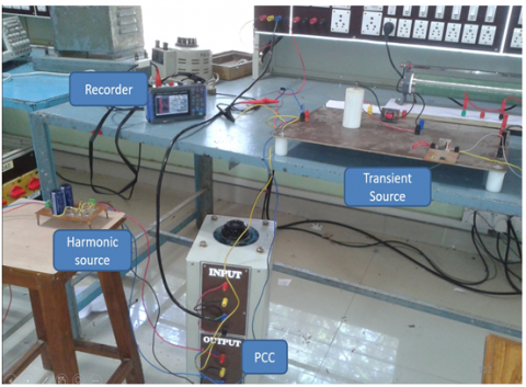
Finally the proposed technique is applied to the real signals acquired by the laboratory experimentation for estimation. Three illustrative voltage signals containing harmonics (A), voltage sag (B) and oscillatory transients (C) simultaneously, are acquired. Figure 14 shows an experimental setup used for laboratory simulation of PCC.
A three phase uncontrolled rectifier with a resistive load is used as harmonic producing source A. Single line to ground fault is created by short circuiting, to produce a voltage sag (i.e. source B). Source C; i.e. transients are produced by switching a capacitor bank. All three disturbance sources are fed by the same supply point; i.e. PCC. HIOKI 8870-20 MEMORY HiCORDER© is used for the signal acquisition. The signals are acquired with 20 kHz sampling frequency.
The acquired signals are processed with the filtering operation as explained and IFFV(τ) are calculated. Table 11 summarizes the results. It can be observed here that the proposed method shows the estimated peak and average values are similar to those calculated by the simulated signals. In the presence of transient disturbances, the peak approaches to thousands and averages are less than hundreds.
Figure 14. Experimental setup of laboratory PCC for signal data acquisition
Table 11. Estimated peak and average values of IFFV(τ) for real PCC voltage acquired by laboratory experimentation
|
Signal Number |
1 |
2 |
3 |
|
|
ABC |
Peak |
1684.97 |
2284.50 |
2864.73 |
|
Average |
142.85 |
141.24 |
141.12 |
|
|
A |
Peak |
306.66 |
326.53 |
683.84 |
|
Average |
51.55 |
46.59 |
68.35 |
|
|
B |
Peak |
210.83 |
174.26 |
88.58 |
|
Average |
115.53 |
98.08 |
34.89 |
|
|
C |
Peak |
1358.03 |
2006.34 |
2462.55 |
|
Average |
36.51 |
39.10 |
38.40 |
|
A method for quantification of the consumer’s responsibility in overall PQ deterioration at the PCC is proposed and verified with the most frequent PQ disturbance sources varied in all possible ways. The method accounts both stationary and non-stationary disturbances.
The IFF(τ) of PCC voltage signal and current signals are used to identify the specific feeder on which the PQ disturbance source of respective disturbance type is located. The results confirm the usefulness of IFF(τ) for the purpose; although the authors suggest the use of intelligent PQ classification algorithms for the same.
Finally, the proposed technique is used for the quantification of the responsibility of individual source to cause the disturbance at the PCC voltage signal. The results show that by using proposed method it is possible to quantify the responsibility of individual consumer, to cause PQ deterioration at PCC, only by analyzing the PCC voltage signal. The method is also applied to real signals acquired by the laboratory PCC for the further validation. The proposed method can be further extended by considering the consumer loads causing various PQ events as defined by IEEE 1159 standards acting on the same PCC.
[1] Hunter, I. (2001). Power quality issues-a distribution company perspective. Power Engineering Journal, 15: 75-80. https://doi.org/10.1049/pe:20010203
[2] Billinton, R., Pan, Z.M. (2002). Incorporating reliability index probability distributions in performance based regulation. Canadian Conference on Electrical and Computer Engineering, 1: 12-17. https://doi.org/10.1109/CCECE.2002.1015167
[3] IEEE Standards 519-1992. (1992). IEEE Recommended Practices and Requirements for Harmonic Control in Electrical Power Systems. https://doi.org/10.1109/IEEESTD.1993.114370
[4] Heydt, G.T., Jewell, W.T. (1998). Pitfalls of electric power quality indices. IEEE Trans. on Power Delivery 13: 570-578. https://doi.org/10.1109/61.660930
[5] IEEE Standards 1159-2009. (2009). IEEE Recommended Practice for Monitoring Electric Power Quality. https://doi.org/10.1109/IEEESTD.2009.5154067
[6] Xu, W., Liu, Y.L. (2000). A method for determining customer and utility harmonic contributions at the point of common coupling. IEEE Trans. on Power Delivery 15(2): 804-811. https://doi.org/10.1109/61.853023
[7] Nath, S., Sinha, P., Goswami, S.K. (2012). A wavelet based novel method for the detection of harmonic sources in power systems. International Journal of Electrical Power & Energy Systems, 40: 54-61. https://doi.org/10.1016/j.ijepes.2012.02.005
[8] de Andrade Jr., G.V., Naidu, S.R., Neri, M.G.G., da Costa, E.G. (2009). Estimation of the utility's and consumer's contribution to harmonic distortion. IEEE Trans. on Instru. and Meas., 58(11): 3817-3823. https://doi.org/10.1109/IMTC.2007.379201
[9] Ferrero, A., Prioli, M., Salicone, S. (2011). Fuzzy metrology-sound approach to the identification of sources injecting periodic disturbances in electric networks. IEEE Trans. on Instru. and Meas., 60(9): 3007-3017. https://doi.org/10.1109/AMPS.2010.5609323
[10] Cataliotti, A., Cosentino, V. (2009). Disturbing load identification in power systems: A single-point time-domain method based on IEEE 1459–2000. IEEE Trans. on Instru. and Meas., 58(5): 1436-1445. https://ieeexplore.ieee.org/document/4787046
[11] Ferrero, A., Salicone, S., Todeschini, G. (2006). Measurement uncertainty role in the identification of the sources of periodic disturbances. 7th Int. Workshop Power Definitions Meas. Nonsinusoidal Conditions, Cagliari, Italy, Jul. 10-12, pp. 66-72.
[12] Parsons, A.C., Grady, W.M., Powers, E.J., Soward, J.C. (2000). A direction finder for power quality disturbances based upon disturbance power and energy. IEEE Trans. on Power Delivery, 15: 1081-1086. https://doi.org/10.1109/ICHQP.1998.760129
[13] Chang, G.W., Chao, J.P., Huang, H.M., Chen, I.C., Chu, S.Y. (2008). On tracking the source location of voltage sags and utility shunt capacitor switching transients. IEEE Trans. on Power Delivery, 23: 2124-2131. https://doi.org/10.1109/TPWRD.2008.923143
[14] Moradi, M.H., Mohammadi, Y. (2012). Voltage sag source location: A review with introduction of a new method. International Journal of Electrical Power & Energy Systems, 43: 29-39. https://doi.org/10.1016/j.ijepes.2012.04.041
[15] Gao, J., Li, Q.Z., Wang, J. (2011). Method for voltage sag disturbance source location by the real current component. In Power and Energy Engineering Conference (APPEEC), 2011 Asia-Pacific, pp. 1-4.
[16] Ma, L. (2017). Evaluation of criticality and vulnerability of busbar based on voltage dip. AMSE JOURNALS-AMSE IIETA publication-2017-Series: Modelling A; 90(1): 85-97. https://doi.org/10.18280/mmc_a.900107
[17] Jaramillo, S.H., Heydt, G.T., O'Neill-Carrillo, E. (2000). Power quality indices for aperiodic voltages and currents. IEEE Trans. on Power Delivery, 15: 784-790. https://doi.org/10.1109/61.853020
[18] Morsi, W.G., El-Hawary, M.E. (2010). Novel power quality indices based on wavelet packet transform for non-stationary sinusoidal and non-sinusoidal disturbances. Electric Power Systems Research, 80: 753-759. https://doi.org/10.1016/j.epsr.2009.11.005
[19] Kandil, M.S., Farghal, S.A., Elmitwally, A. (2001). Refined power quality indices. IEE Proceedings -Generation, Transmission and Distribution, 148: 590-596.
[20] Morsi, W.G., El-Hawary, M.E. (2001). Power quality evaluation in smart grids considering modern distortion in electric power systems. Electric Power Systems Research, 81: 1117-1123. https://doi.org/10.1016/j.epsr.2010.12.013
[21] Shin, Y.J., Powers, E.J., Grady, M., Arapostathis, A. (2006). Power quality indices for transient disturbances. IEEE Trans. on Power Delivery, 21: 253-261. https://doi.org/10.1109/TPWRD.2005.855444
[22] Jia, Y., He, Z.Y., Zang, T.L. (2010). S-transform based power quality indices for transient disturbances. In Power and Energy Engineering Conference (APPEEC), 2010 Asia-Pacific, pp. 1-4.
[23] Uyar, M., Yildirim, S., Gencoglu, M.T. (2009). An expert system based on S-transform and neural network for automatic classification of power quality disturbances. Expert Systems with Applications, 36: 5962-5975. https://doi.org/10.1016/j.eswa.2008.07.030
[24] Naik, C.A., Kundu, P. (2014). Power quality disturbance classification employing S-transform and three-module artificial neural network. International Transactions on Electrical Energy Systems, 24: 1301-1322. https://doi.org/10.1002/etep.1778
[25] Polikar, R., Udpa, L., Udpa, S.S., Taylor, T. (1998). Frequency invariant classification of ultrasonic weld inspection signals. IEEE Trans. on Ultrasonics, Ferroelectrics and Frequency Control, 45: 614-625. https://doi.org/10.1109/58.677606
[26] Naik, C.A, Kundu, P. (2012). New power quality indices based on S-transform for non-stationary signals. In Proc. Int. conf. of power and energy PECON 2012, pp. 677-682. https://doi.org/10.1109/PECon.2012.6450301
[27] Stockwell, R.G., Mansinha, L., Lowe, R.P. (1996). Localization of the complex spectrum: The S-transform. IEEE Trans. on Signal Processing, 44(4): 998-1001. https://doi.org/10.1109/78.492555