A. Samson Myles* | O. Savadogo† | Kentaro Oishi
OPEN ACCESS
This paper discusses concept of a novel Building Integrated Photovoltaic-Thermal (BIPV-T) solar module (collector). The concept proposes uniform water cooling of individual solar cells in a module to improve performance of photovoltaic (PV) modules. A simulation study was conduct-ed using TRNSYS software that shows much improvement in performance of PV module if individual cells could be cooled separately. Based on our analysis, a novel concept of a cooling pipe layout (heat exchanger) is proposed that will improve the performance of overall energy efficiency of the PV module over conventionally used series cooling of solar cells in BIPV-T modules. This will help to open a new design of BIPV-T technology based on our proposed BIPV-T module.
When a PV module is flush with the roof or wall of a building, its natural cooling from back of PV module is impeded (Sandia) [1]. That means when ambient temperature is 25°C, solar cell temperature will increase to 45°C (NOCT) + 18°C = 63°C. In warmer climates than 25°C, the cell temperature will be higher than 63°C, thereby reducing the power output substantially.
In the past, researchers have tried many different matrixes for cool-ing PV modules [2-14]. Unfortunately, each configuration which has been tried so far causes non-uniform cooling of individual solar cells in a module. Various cooling pipe layout proposed in the past [15] suffer from major disadvantage that solar cells used within a solar module will operate at different temperatures thereby achieving less benefit [15]. They do not integrate circulation of cooling water at indi-vidual cell level and this impacts negatively the electrical performance of the BIPV-T system.
As the temperature of the cooling water picks up heat starting at first solar cells at inlet, its temperature continue to rise. As the cooling wa-ter flows, solar cells next in order for cooling receives higher tempera-ture than first solar cells Figure 1 depending on cooling pipe configu-ration. Hence the drop in voltage of the solar cells in module will in-crease as its temperature rises and efficiency will be lower. Though current output increases slightly at higher temperatures, it does not contribute in increasing power output. However, with the temperature increase, voltage decreases more significantly than the increase in current in same conditions.
This is because current generated by solar cells at lowest tempera-ture will be the final output current for the module. This progressive increase in the cell temperature appears when the water flows from the first cell at the inlet to the last cell at the outlet. For example, the cur-rent coefficient is in the order of the +0.04% and those of voltage is -0.4%. The solar module voltage drops significantly when its tempera-ture increases. To solve this problem, we suggest in this work to devel-op a novel cooling system based on individual cell cooling to extract maximum heat from the BIPV-T module to maximize electrical out-put.
Accordingly, first, we will use TRNSYS to design a new configura-tion of a BIPV-T water cooling path. Secondly, we simulate the ther-mal behaviour of the module using different water flow rates through individual cell. The simulated results will be compared to those of classic parallel tube flow cooling design. Thirdly, we will analyse the thermal behaviour of the BIPV-T obtained in this work to those of the parallel tube type cooling system.
Based on the TRNSYS simulation model, the following equation is shown for the energy balance on the photovoltaic panel neglecting conduction along the surface [8]:
$\mathbf{0}=S-\boldsymbol{h}_{\text {outer }}\left(T_{P V}-\boldsymbol{T}_{a m b}\right)-\boldsymbol{h}_{\text {rad }}\left(T_{P V}-\boldsymbol{T}_{s k y}\right)-\frac{T_{P V}-T_{a b s}}{R_{T}}$ (1)
where,
$\mathbf{S}[k J / h r]-$ The net absorbed solar radiation (total absorbed PV power production)
$\mathbf{h}_{\text {outer }}\left[\mathrm{kJ} / \mathrm{hr} \cdot \mathrm{m}^{2} \cdot \mathrm{K}\right]-$ The heat transfer coefficient from top of the PV module surface to ambient air;
$\mathbf{T}_{\mathrm{PV}}\left[{ }^{\circ} \mathrm{C}\right]-$ The PV cell temperature
$\mathbf{T}_{\mathrm{amb}}\left[{ }^{\circ} \mathrm{C}\right]-$ The ambient temperature for convective losses from top surface
$\mathbf{h}_{\mathrm{rad}}\left[\mathrm{kJ} / \mathrm{hr} \cdot \mathrm{m}^{2} \cdot \mathrm{K}\right]-$ The radiative heat transfer coefficient from the top of PV surface to the sky
$\mathbf{T}_{\mathrm{abs}}\left[{ }^{\circ} \mathrm{C}\right]-$ The PV surface temperature (absorber temperature)
$\mathbf{R}_{\mathbf{T}}\left[\mathrm{h} \cdot \mathrm{m}^{2} \cdot \mathrm{K} / \mathrm{k} \mathrm{J}\right]-$ The resistance to heat transfer from PV cells to the absorber plate at the back
The PV power output can be calculated as [8]:
$P V_{\text {power}}\left[\frac{\mathrm{kJ}}{\mathrm{hr}}\right]=(\tau \alpha)_{n} \cdot I A M \cdot G_{T} \cdot A_{P V} \cdot \eta_{P V}$ (2)
where,
$(\mathrm{T} \alpha)_{\mathrm{n}}-$ The transmission-absorptance product for the PV module at normal incidence
IAM – Incidence angle modifier
$\mathbf{G}_{\mathbf{T}}\left[\mathbf{k} \mathbf{J} / \mathrm{hr} \cdot \mathbf{m}^{2}\right]$ – The total solar radiation incident upon the surface of BIPV-T module
From the relation (2), $\eta_{P V}$ the module efficiency is very sensitive to the temperature variations. Efficiency $\eta_{P V}$ can be expressed by
$\boldsymbol{\eta}_{P V}=Efficiency of PV module=\eta_{\text {nominal}} \cdot X_{\text {CellTemp}} \cdot X_{\text {Radiation}}$ (3)
where,
$\boldsymbol{\eta}_{\text {nominal}}$ is the module efficiency at standard test condition (STC)
$X_{\text {CellTemp}}\left[1 /{ }^{\circ} \mathrm{C}\right]=\mathbf{1}+\operatorname{Eff}_{T}\left(\boldsymbol{T}_{P V}-\boldsymbol{T}_{\text {ref}}\right)$ (4)
$X_{\text {CellTemp}}$ is the multiplier for PV cells efficiency is a function of the temperature
$\boldsymbol{X}_{\text {Radiation}}\left[h . m^{2} / k J\right]=\mathbf{1}+\operatorname{Eff}_{\boldsymbol{G}}\left(\boldsymbol{G}_{T}-\boldsymbol{G}_{\text {ref}}\right)$ (5)
$X_{\text {Radiation}}$ is the multiplier of radiation,
where,
$G_{\text {ref}}$ is $1000 \mathrm{W} / \mathrm{m}^{2}\left(3600 \mathrm{kJ} / \mathrm{hr} \cdot \mathrm{m}^{2}\right)$
$\mathrm{Eff}_{T}$ is the module temperature coefficient. This coefficient is always negative, and its value depends on the module technology.
In this work: $\mathbf{E f f}_{T}=-0.0048[1 / \mathrm{C}]$ and $\mathbf{E f f}_{G}=$ is $2.5 \times 10^{-5}\left[\mathrm{h} \cdot \mathrm{m}^{2} / \mathrm{kJ}\right]$
The thermal output of the BIPV-T module can be calculated as [8,9]
$\boldsymbol{Q}_{\boldsymbol{u}}=\boldsymbol{m} \cdot \boldsymbol{C}_{p}\left(\boldsymbol{T}_{\text {fluid}, \text {out}}-\boldsymbol{T}_{\text {fluid}, \text {in}}\right)$ (6)
where,
$C p[\mathrm{kJ} / \mathrm{kg} . \mathrm{K}]-$ The specific heat of the fluid flowing through the BIPV-T collector
$Q_{u}[\mathrm{kJ} / \mathrm{hr}]-$ The rate at which energy is added to the flow stream by the BIPV-T module
$m[\mathrm{kg} / \mathrm{hr}]-$ The flow rate of fluid through the collector of the BIPVT module
$T_{\text {fluid}, \text {out}}\left[{ }^{\circ} \mathrm{C}\right]-$ The temperature of fluid flowing out of the BIPV-T module
The thermal efficiency of BIPV-T module can be calculated as follows [8, 9]:
$\boldsymbol{\eta}_{t h e r m a l}=\frac{Q_{u}}{G_{T} \cdot A_{P V}}$ (7)
Based on these above concepts, the input parameters used to achieve TRNSYS Simulation are indicated in Table 1. We use a solar module of 1.483m length and 0.665m width. In the designed prototype the collector length is 1.466m and width 0.66m. The absorber plate is made of copper sheet to paste at the back of the module. Its thickness is 0.0005m and the thermal conductivity is given by the supplier is 1386kJ/hr.m.K (385W/m.K). For each solar cells we used 2 tubes in contact with copper sheet to circulate water to collect heat. The diameter of each tube is 0.03m. The contact (bond) width between plate and to be is taken as 0.01m whereas bond thickness is taken as 0.01925m. The bond thickness (th) is calculated from the simple relation,
$\boldsymbol{t h}=\frac{c_{b}}{\left(k_{b} \boldsymbol{b}\right)}$ (8)
Where, $c_{b}$ is the copper sheet and tube interface conductance, $k_{b}$ is the bond thermal conductivity and $b$ is the bond width. In our case $c_{b}=$ $200 \mathrm{W} / \mathrm{mk}, k_{b}=1386 \mathrm{kJ} / \mathrm{hmk}$ and $b=0.01 \mathrm{m}$
The thermal resistance of the substrate is calculated as
$\frac{\text {Total thickness of PV laminate material}}{\text {Mean thermal conductivity of PV laminate material}}$
The total thickness of PV laminate is $0.00818 \mathrm{m}$ and mean thermal conductivity of PV laminate material [4] is taken as $136.7 \mathrm{W} / \mathrm{mK}$ Therefore, the thermal resistance works out to $6 \times 10^{-5} \mathrm{m}^{2} \mathrm{K} / \mathrm{W}\left(1.7 \mathrm{x} 10^{-}\right.$ $\left.{ }^{5} \mathrm{m}^{2} \mathrm{K} / \mathrm{kJ}\right)$
The resistance of the back insulation is taken as $1 \times 10^{-4} \mathrm{hm}^{2} \mathrm{K} / \mathrm{kJ}$ from manufacturers data, the reflectance is calculated as ( 1 - (glass trans-mittance x cell absorptance)) where transmittance of the glass is taken as 0.9 and the absorptance of the cell is taken as $0.9 .$ Therefore, the reflectance works out to $(1-0.9 \times 0.9)=0.19$.
IAM is the incidence angle modifier and is calculated from following equation
$K_{\tau \alpha}=1-b_{0}\left(\left(\frac{1}{\cos \theta}-1\right)^{n}\right.$ (9)
where $b_{0}$ is the incidence modifier coefficient and $n$ is a constant specific to type of coating on the absorber. In our study for a flat cover $n$ is taken as 1.
The PV reference temperature is taken as $25^{\circ} \mathrm{C}$ which is the reference temperature define for the PV performance under standard test condition (STC). The PV cell reference radiation of $3600 \mathrm{kJ} / \mathrm{hr} \cdot \mathrm{m}^{2}$ (or $\left.1000 \mathrm{W} / \mathrm{m}^{2}\right)$ is the same as solar radiation used for testing PV module under standard test condition (STC). The PV efficiency at reference condition is once again efficiency of PV module at STC. In our case it is taken as 0.142 or $(14.2 \%) .$ The efficiency modifier for the temperature is the temperature coefficient for power output of the PV module. This is given by the PV module manufacturer obtained from module certifying authority like TUV or UL. We have used the manufacturers data as -0.0048 (or $0.48 \% /{ }^{\circ} \mathrm{C}$ ). The efficiency modifier for the radiation depends on air mass. It has been neglected as the modules are tested at near noon time when the air mass is close to 1.
3.1 Conventional BIPV-T cooling circuit analysis
Figure 1 shows the how conventional cooling circuits for BIPV-T or PV-T modules are used [1, 3, 5, 8]. Infact, various cooling circuit (cooling pipe layout) proposed such as parallel flow [3, 5, 8], split flow [2], direct flow [2], spiral flow, parallel serpentine [2], web flow, duel pass, drip flow, oscillatory flow etc. All these concepts could be explained through Figure 1. All these flow models are characterized by one inlet fluid flow through the panel to one output fluid flow. In this case the same fluid goes in one line from a cell to another cell of the panel. In other words we take one string of cells which is shown in Figure 1, we see that the same cooling fluid is going from cell1 to cell 9. In such configuration the temperature of cell 9 will higher then temperature of cell1. The Figure 1 outlet temperature of cooling fluid from cell1 is denoted as t1 and outlet temperature of fluid at the exit of cell 9 is denoted as t9 where t9 > t1. Therefore, in this cooling pipe configuration the temperature of the cells in a module cannot be uniform.
Figure 1. Conventional BIPV-T and PV-T cooling pipe layout
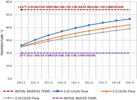
Using the experimental parameters tabulated in Table 1 for running TRNSYS simulation, Figure 2 shows the variation of each cell temperature with the number of the cell; from no1, the number of the first cell which receives the inlet of the flow rate to no9 the number of the last cell from which we have the outlet of the flow rate result for 9 series connected solar cells in a 4 x 9 (36 cell) solar modules. The temperature increases from cell no1 to cell no9 for a given flow rate. For a fixed number of cells, the temperature of the cell decreases when the fluid rate through the panel increases.
Table 1. Input parameters for simulation using TRNSYS software
|
S.N |
DESCRIPTION |
VALUE |
UNIT |
|
1 |
Collector length |
1.483 |
m |
|
2 |
Collector width |
0.665 |
m |
|
3 |
Absorber plate thickness |
0.0005 |
m (24 gage) |
|
4 |
Thermal conductivity of the absorber |
1386 |
kJ/hr·m·K |
|
5 |
Number of tubes |
8 |
- |
|
6 |
Tube diameter |
0.03 |
m |
|
7 |
Bond width |
0.01 |
m |
|
8 |
Bond thickness |
0.01925 |
m |
|
9 |
Bond thermal conductivity |
1386 |
kJ/hr·m·K |
|
10 |
Resistance of substrate material |
0.000017 |
h·m2·K/kJ |
|
11 |
Resistance of back material |
R6.7 |
h·m2·K/kJ |
|
12 |
Fluid specific heat |
4.18 |
kJ/kg·K |
|
13 |
Reflectance |
0.19 |
Fraction |
|
14 |
Emissivity |
0.9 |
Fraction |
|
15 |
1st order IAM (b0) |
0.136 |
- |
|
16 |
PV cell reference temperature |
25 |
°C |
|
17 |
PV cell reference radiation |
3600 |
kJ/hr·m2 |
|
18 |
PV efficiency at reference condition |
0.175 |
Fraction |
|
19 |
Efficiency modifier - temperature |
-0.0048 |
1/°C |
|
20 |
Efficiency modifier - radiation |
0 |
h·m2/kJ |
NOTE: To determine the flow rate for simulation reference EUROFINS, Italy [5] and TUV Reinland [6] which is conducted outdoors and indoors respectively.
These results are in agreement with those published elsewhere by Zondag H. A., et al., [16] where it was found a progressive increase of the cell temperature from the first cell at the inlet of the fluid flow to the last cell of the outlet of the fluid flow. The thermal efficiency obtained in his work was 33% for combi panel as compared to 54% for conventional thermal panels. Electrical efficiency of Combi panel was found to be 6.7% as compared to 7.2% for conventional PV panels measured in the same condition.
Figure 2 shows how the current output of solar cell increases with temperature. However, it will have negligible effect in output power as cell with lowest cell current output will be the net current output for series connected solar cells.
Figure 2. Simulation results for 9 series connected Solar Cells in a 140W module at varying flow rates for 800W/m2 Solar Radiation, 20°C ambient temperature
For the purpose of explanation and clarity, Figure 1 depicts conventionally made water cooling pipe configuration. A nine cells series connected solar cells are shown. separately for analysis as cooling water will get divided in four parallel paths. Therefore, the performance of each 9 series connected solar cells will be identical but non-uniform.
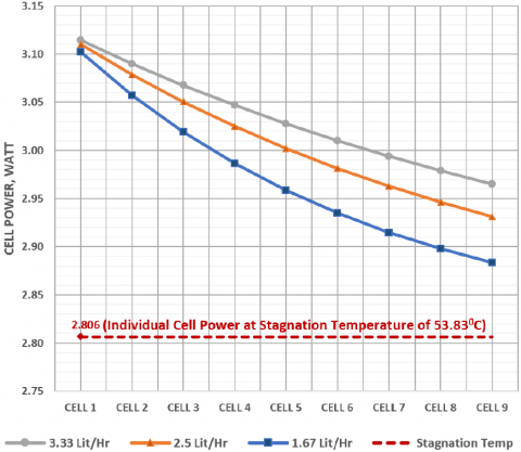
Figure 3 shows the variation of the wattage power with the number of the cell. When the cell number increases the cell wattage power decreases. From the cell no 1 to cell no 9, the drop in the power increases when the flow rate decreases for each cell. This results in power drop of solar cell indicates that power output of each cell will be different. The net effect of this cooling scheme is a limited increase in output power of solar modules. But the performance in power of the module is significantly worst without cooling. As shown in Figure 3, the power of each of the 9 cells will vary as the cooling water moves from one solar cell to next. The graph also shows that first cells will have higher pow-er where cooling water enters the cooling circuit. When compared to the power of the non cooled system which temperature will rise to 53.83°C, the power drops to 2.806 W whereas the cooled first cell has a voltage of 3.102 W at a flow rate of 1.67/litres per hour. With this watt-age at 53.83°C used for comparison, the gap of the wattage in the first cell is around 0.300 Volt whereas it is 0.008 Volt for the last cell if the water cooling flow rate is 1.67 litres/hour. In Figure 3, we see that when the water flow rate increases, difference of wattage increases from the situation without cooling (2.806 Watts) to the value of 3.110 Watt for the first cell and is almost independent of the flow rate. But it increases from 0.08 Watt to 0.16 W when the flow rate increases from 1.67 lit/hour to 3.33 lit/hour. This is an indication of the effect of the flow rate on the thermal efficiency of the system. For purpose of the explanation red and violet dotted lines showing cell wattage of 2.806 Wattage at the temperature of 53.830C for not cooled system (stagnation).
Figure 3. Simulation results of individual wattage of nine series connected Solar Cells at varying cooling water flow rates for 800W/m2 solar radiation and 20°C ambient temperature
Simulation of the variation of the wattage power with the number of the cell for a created for a 36-cell 140W polycrystalline module. Figure 3 shows the wattage of 9 individual cells connected in series. Each cell will operate at different wattages mainly because voltage of solar cells drops as the temperature of cells rises. For reference, the power output of solar cell at stagnation temperature is shown in red.
3.2 Concept and new design of cooling water circuit
In order to understand the new concept refer to graphical perfor-mance shown in Figure 4, Table 2 and Table 3 below.
Figure 4. Individual Cell Cooling of 9 series cells using novel water cooling pipe layout
Table 2. Performance of PV module at varying cooling water flow rates. The cooling is based on flowing cooling water over none cells in a row versus individual solar cells using at 800W/m2 & 20°C ambient.
|
Flow rate |
140W, 36 cell module wattage |
Individual cell gain % |
Gain over Stagnation % |
||
|
lit/hr |
Series cooling |
Individual cell uniform cooling |
Gain over series cells |
||
|
1.67 |
107.02 |
111.68 |
4.66 |
4.35% |
10.53% |
|
2.50 |
108.35 |
111.96 |
3.61 |
3.34% |
10.82% |
|
3.33 |
109.18 |
112.11 |
2.93 |
2.69% |
10.96% |
|
0.00 |
101.03 |
101.03 |
0.00 |
0.00% |
0.00% |
NOTE: cooling water inlet temperature 20°C
Table 3. Electrical & thermal efficiency of BIPV-T module for cooling by passing water over nine cells in a row versus individual cell cooling
|
Flow rate |
Series cells cooling Module |
Individual cell uniform cooling |
||||
|
lit/hr |
PV Eff % |
Therm Eff % |
Overall Eff % |
PV eff % |
Therm Eff % |
Overall Eff% |
|
1.67 |
13.38 |
25.22 |
38.60 |
13.96% |
45.21% |
59.17% |
|
2.50 |
13.54 |
30.44 |
43.98 |
14.00% |
46.36% |
60.36% |
|
3.33 |
13.65 |
33.60 |
47.25 |
14.01% |
46.95% |
60.96% |
|
0.00 |
12.63 |
0.00 |
12.63 |
12.63% |
0.00% |
12.63% |
As seen in Figure 5, a sub header 2 water input pipe is placed along the length of 9 cells to feed cooling water in individual cells. On the otherside of cells width another outlet header pipe 2 is use to collect hot water after water picks up heat from each solar cells. This design re-quires additional feeder(inlet) and outlet pipes to feed the sub-headerpipes along the cells. Similarly, additional sub-header pipe for taking out the heated water is connected to main hot water outlet header pipe. It is made sure, header pipes do not touch any solar cells to transfer heat.
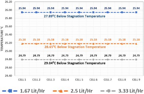
The analysis clearly indicates that if all solar cells in a BIPV-T or PV-T modules are cooled uniformly at same temperature we can get achieve high module output. At higher cooling water flow rate the cell temperatures are lower and temperature rises at lower flow rates. Also noticeable is that higher or lower cooling water flow rates there is in-significant variation in temperature and output gain. The main ad-vantage of new cooling pipe configuration is that even at higher tem-peratures all solar cells can be maintained at uniform temperature.
Figure 4 graph shows the cooling effect of different water flow rates. A BIPV-T solar module will operate 28 to 29°C below the stagnation temperature of solar cells. The power and efficiency gains are shown in Table 2 and Table 3.
Figure 2 show the variation of the cell temperature with the number of cells for the same water cooling flow rates as for Figure 3. A same constant temperature of the cell is obtained from the first to the last cell. For the same flow rate. This indicated that each cell of the panel has the same temperature prior to the individual cooling.
Figure 4 depicts lowest cell temperature for all cells if cooling water enters and exits from individual cells. Combining Figure 3 and Figure 4. shows if all solar cells have same temperature as the first cell then we can get highest power output from each cell. For example at 1.67lph flow rate all cells will deliver 3.102W (1st Cell) x 9 cells = 27.92W if they operating at uniform temperature same as first cell. For non-uniform cooling combining the strings of 9 will deliver 2.883W (9th Cell) x 9 cells = 25.95W. The higher power generated by other 8 cells will be dissipated in the 9th cells until the current output of all cells become equal. Therefore, uniformly cooled individual cells will deliver 7.6% higher power.
Table 2 and Table 3 show clearly an important wattage gain over the series cooling with and individual cell gain of 4,35 % for a flow rate of 1,67 lit/hr and a gain over stagnation about 10,5% for the same flow rate.. there is not a significant gain over stagnation with the flow rate increases.
Based on the improved performance results for individual cell cool-ing in a module, a novel cooling coil layout was designed as shown in Figure 5.
Figure 5. Design of a 36 cell BIPV-T solar module with a novel cooling pipe layout. This individual cooling system has never been developed before and it better perfornace than previous cooling system are not individually cooled.
Figure 5 Shows our proposal for a new design of a 36 cell BIPV-T solar module with novel cooling pipe layout. In the actual prototype a copper sheet attached to cooling water tube is pasted at the back of standard commercially available solar module. The cold and hot water headers (depicted in blue and red in Figure 5) are higher than riser pipes (depicted in orange) to prevent the former from touching the solar cells.
In this case as shown in Figure 5 we have main input header pipe 1 where cooling water enters and distributes cooling water to three input sub-headers 2. Each sub-header pipe 2 then feeds cooling water to riser tubes (Figure 5) to cool individual cells. The outlet sub-header pipe 2 is provided on the otherside of individual cells to collect warm fluid which picks up heat from each cell. This cooling pipe configuration ensures uniform temperature of individual solar cells in the modules. The two outlet sub-headers pipe 3 connects to main header pipe 1 for warm water to exit from the module. The results obtained from the TRNSYS and experimental meausrements made on a protype based on individual cell cooling we will fabricate to show an important improve-ment of the cooling system in comparison of the other previous cooling system.
The fabricated BIPV-T prototype is expected to have following im-provements over water cooling pipe configurated used by other re-searchers
1. All 36 solar cells in BIPV-T module will operate at uniform temper-ature with minimum variation.
2. The mismatching of solar cells electrical output will be minimised which will improve efficiency.
3. The even cooling will prevent overheating of any solar cells that causes premature failure of modules.
4. The overall efficiency will increase due to heat gain in cooling wa-ter. The combined thermal and electrical efficiency will boost over-all efficiency of BIPV-T module.
The TRNSYS simulation results shows approximately 10.5% to 11% improvements in performance of BIPV-T modules using novel water-cooling circuit over conventional BIPV modules. In addition, the simu-lation indicates that novel cooling circuit layout will have 3.2% to 4.3% improvement over BIPV-T modules with series cooling proposed by some researchers and commercially available from some manufactur-ers. Additionally, thermal efficiency between 45% to 47% is achieved by collecting heat in cooling water.
The novel design prevents negative effect of non-uniform cooling of solar cells in a module. In conventional cooling pipe configuration used in other studies will generated highest current by hottest cells at the outlet. Since all cells in modules are connected in series, the cells at the inlet will operate at lowest temperature and higher current generated by cells at higher temperature will get absorbed this cell. This can cause overheating of cell/cells that generate lower current. As PV technology is progressing fast, solar cells are generating higher currents year after year. This means current mismatching can have more severe effect.
The uniform cooling of individual cells proposed here will ensure mismatching of current does occur.
Infact, BIPV-T modules with glazing will have more severe effect in mismatching as the solar cell operate at even higher temperature. The uniform cooling even at higher water temperature, as shown in graph Figure 4 and novel cooling pipe layout shown in Figure 5, will have major advantage in keeping the solar cells at uniform temperatures.
Though this study was conducted for water based cooling system same concept of uniformly cooling individual cell could be applied to air cooling system in BIPV-T modules.
A BIPV-T module design based on cooling of individual solar cells was constructed and tested outdoors in natural sunlight. In next paper, complete design and fabrication details as well as test result of proto-type is discussed.
[1] M. K. Fuentes, "A simplified thermal model for flat-plate photovol-taic arrays," Sandia National Labs., Albuquerque, NM (USA), 1987.
[2] M. Y. Othman, A. Ibrahim, G. L. Jin, M. H. Ruslan, and K. Sopian, Renewable Energy, 49, 171 (2013).
[3] "Hybrid PV-Thermal Data Sheet," ed: Solimpeks, 2013.
[4] T. T. Chow, Applied energy, 87, 365 (2010).
[5] "Test Report M1.11.NRG.0320/43724: Volther Powervolt," Euro-fins, Italy, August 2011.
[6] "Test Report 21222892_E: DualSun 250M," TUV Reinland Ener-gie und Umwelt GmbH, November 2013.
[7] V. Tyagi, S. Kaushik, and S. Tyagi, Renewable and Sustainable Energy Reviews, 16(3), 1383 (2012).
[8] J. A. Duffie and W. A. Beckman, Solar engineering of thermal processes. John Wiley & Sons, 2013.
[9] Stine, W. B., and G. Michael, "Power from the Sun," ed, 2001.
[10] T. N. Anderson, M. Duke, G. L. Morrison, and J. K. Carson, Solar Energy, 83(4), 445 (2009).
[11] T. N. Anderson, S. K. Bura, M. Duke, J. K. Carson, and M. C. Lay, "Development of a building integrated photovoltaic/thermal solar collector based on steel roofing," 4th New Zealand Metals Industry Conference, 2008.
[12] Y. Tripanagnostopoulos, Solar energy, 81(9), 1117 (2007).
[13] M. Bosanac, B. Sorensen, K. Ivan, H. Sorensen, N. Bruno, and B. Jamal, "Photovoltaic/thermal solar collectors and their potential in Denmark," Final Report, EFP Project, www. solenergi. dk/rapporter/pvtpotentialindenmark. pdf, 2003.
[14] V. J. Fesharaki, M. Dehghani, J. J. Fesharaki, and H. Tavasoli, , "The effect of temperature on photovoltaic cell efficiency," in Proceedings of the 1stInternational Conference on Emerging Trends in Energy Conservation–ETEC, Tehran, Iran, 2011, pp. 20-21.
[15] T. Matuska, "Theoretical analysis of solar unglazed hybrid photo-voltaic-thermal liquid collector," in Proceedings of the Eurosun, 2010.
[16] H. A. Zondag, D. d. de Vries, W. Van Helden, R. C. van Zolingen, and A. Van Steenhoven, Solar energy, 72(2), 113 (2002).