Abderrahmane Berkani* | Mohamed Bey | Rabah Araria | Tayeb Allaoui
© 2020 IIETA. This article is published by IIETA and is licensed under the CC BY 4.0 license (http://creativecommons.org/licenses/by/4.0/).
OPEN ACCESS
In order to perform the control of a voltage source converter and enhance its capability of working, in this work, a new approach based on Fuzzy-Q-Learning algorithm is applied. The utilized method makes the fuzzy controller in dynamic mode that means this controller will be adapted in each variation in the system by changing the different values depends on the change in the system. By perform the DPC technique, the obtained results show that this new fuzzy reinforcement gives better performance to control a voltage source converter.
Fuzzy-Q-Learning (FQL), Direct Power Control (DPC), Fuzzy Logic Control (FLC), Voltage Source Converter (VSC)
Conventional tuning methods are based on adequate modeling of the system to be tuned and analytical processing using the transfer function or equations of state. Unfortunately, these are not always available. These control techniques have proven their effectiveness in many industrial regulation problems. Advanced control methods (Adaptive Controller, Predictive Control, Robust Control ...) meet the requirements of a number of highly non-linear systems. It is in this same deal that the fuzzy modeling and control methods are positioned [1]. The majority of complex industrial systems such as the voltage source converter are difficult to control automatically. This difficulty arises from: - their non-linearity, - the variation of their parameters, - the quality of the measurable variables. These difficulties have led to the advent and development of new techniques such as fuzzy control, which is particularly interesting when there is no precise mathematical model of the process to be controlled or when the latter presents strong nonlinearities or imprecisions [2]. In many applications of VSC controller, the results obtained with a fuzzy controller are better than those obtained with a conventional control algorithm. In particular, the fuzzy control methodology appears useful when the processes are very complex to analyze by conventional techniques. Several works in the field of VSC control have shown that a fuzzy logic regulator is more robust than a conventional regulator.
Despite this performance of fuzzy logic, it remains limited in the case of dynamic systems, a change of a parameter or an external disturbance can affect the functioning of this system, and so, even the technique of fuzzy logic requires an improvement. In this context, H.R. Berenji proposes a reinforcement of this technique; it is the Fuzzy Q-learning approach [3, 4]. The principal of this last one, which make the fuzzy controller in dynamic mode, will be detailed in the next section
By investigating in the quality of this approach, and using Direct Power Control (DPC) [5, 6], in this work, we analyzed the effect of this combination in helping a VSC to work properly.
In the same objective, not just the technic of control it performed but the structure of the VSC also has been changed, for that, a 3 level T-type VSC converter represent the studied system [7].
This paper is organized as follows: in Section 2, three level T-type VSC topology and its modeling are presented. The Proposed fuzzy Q learning direct power control (FQL DPC) is developed in Section 3. The application of the proposed control approach with 3 level DPC technic on the studied VSC is presented in Section 4. Sections 5 describe the simulations results and their discussions and finally conclusions are mentioned in the last section.
Figure 1 shows a T-type three-level converter, where the two capacitors create a midpoint 0. Each capacitor must be sized for a voltage equal to Vdck/2. Each converter arm includes four switching devices and four diodes with an additional active bidirectional switch connected to the midpoint of the DC link [8, 9]. The controlled switches are unidirectional in voltage and bidirectional in current; they are classic associations of a transistor and an anti-parallel diode. The output of an arm of the bridge can be connected to the positive P, neutral 0 or negative N voltage level of the DC link.
By closing Skx1, the neutral level by closing Skx2 and Skx3, and the negative level by closing Skx4, where, x = a, b or c and k = r or i.
If we close not only Skx1, but Skx1 and Skx2 for the positive voltage level, Skx2 and Skx3 for the neutral, and Skx3 and Skx4 for the negative voltage level, the current naturally switches to the correct branch independent of the direction of the current [10].
Table 1, describes the switching states necessary to generate the desired voltage levels. If these switching signals are used, the modulation is identical to the three-level NPC topology modulation [10].
Figure 1. Three-level T-type converter
Table 1. States of an arm of the T-type three-level converter
|
State of arm |
State of switch in the arm |
Output Voltage |
|||
|
Skx1 |
Skx2 |
Skx3 |
Skx4 |
||
|
P |
1 |
1 |
0 |
0 |
+Vdck/2 |
|
0 |
0 |
1 |
1 |
0 |
0 |
|
N |
0 |
0 |
1 |
1 |
-Vdck/2 |
2.1 Modeling of the T-type three-level converter
For each arm of the converter, three connection functions are defined, each of which is associated with one of the three states of the arm, which gives:
$\left\{\begin{array}{l}
F_{k x 2}=S_{k x 2} * S_{k x 1} \\
F_{k x 1}=S_{k x 2} * \overline{S_{k x 1}} \quad x=a, b, c \\
F_{k x 0}=\overline{S_{k x 2}} * S_{k x 1}
\end{array}\right.$ (1)
The potentials of nodes a, b and c of the three-phase three-level inverter with respect to point 0 are given by the following system:
$\left\{\begin{array}{l}
v_{t k a 0}=F_{k a 2}\left(v_{c 2 k}+v_{c k 1}\right)+F_{k a 2} v_{c k 1} \\
v_{t k b 0}=F_{k b 2}\left(v_{c 2 k}+v_{c k 1}\right)+F_{k b 2} v_{c k 1} \\
v_{t k c 0}=F_{k c 2}\left(v_{c 2 k}+v_{c k 1}\right)+F_{k c 2} v_{c k 1}
\end{array}\right.$ (2)
where, C1, 2kv are the voltages across the capacitors.
Phase-to-phase voltages are expressed by:
$\left\{\begin{array}{l}
v_{t k a b}=\left(v_{t k a 0}-v_{t k b 0}\right) \\
v_{t k b c}=\left(v_{t k b 0}-v_{t k c 0}\right) \\
v_{t k c a}=\left(v_{t k c 0}-v_{t k a 0}\right)
\end{array}\right.$ (3)
The output voltages of the arms are expressed by:
$\left[\begin{array}{c}
v_{t k a} \\
v_{t k b} \\
v_{t k c}
\end{array}\right]=\frac{1}{3}\left[\begin{array}{c}
v_{t k a b}-v_{t k c a} \\
v_{t k b c}-v_{t k a b} \\
v_{t k c a}-v_{t k b c}
\end{array}\right]$ (4)
which gives the following model:
$\left[\begin{array}{c}
v_{t k a} \\
v_{t k b} \\
v_{t k c}
\end{array}\right]=A^{*}\left[\begin{array}{c}
v_{c k 2}+v_{c k 1} \\
v_{c k 1}
\end{array}\right]$
$A=\frac{1}{3}\left[\begin{array}{l}
2 F_{k a 2}-F_{k b 2}-F_{k c 2} 2 F_{k a 1}-F_{k b 1}-F_{k c 1} \\
2 F_{k b 2}-F_{k a 2}-F_{k c 2} 2 F_{k b 1}-F_{k a 1}-F_{k c 1} \\
2 F_{k c 2}-F_{k a 2}-F_{k b 2} 2 F_{k c 1}-F_{k b 1}-F_{k a 1}
\end{array}\right]$ (5)
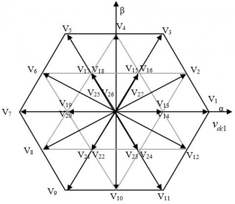
2.2 T-type three-level converter vector diagram
For a three-level converter, there are 18 discrete positions, distributed over two hexagons, in addition to a position in the center of these hexagons. The positions of the output vector in the internal hexagon are created by two redundant states.
The position of the center of these hexagons corresponds to a zero-output voltage, generated by three redundant states [11]. The 19 positions of the output voltage vector divide the vector diagram into six triangular sectors. Each sector is composed of four triangles as shown in Figure 2.
Figure 2. Vector diagram of the T-type three-level converter
2.3 Three-level T-type rectifier modeling
Figure 3 consists of a three-level type T rectifier connected to the AC network via a line filter Rr, Lr.
The DC output bus is made up of two capacitors in series. The total DC bus voltage is Vdcr. under normal operating conditions; this is uniformly distributed over the two capacitors, which then have a voltage Vdcr/2 at their terminals.
The mathematical equations, which govern the dynamic behavior of the voltages on the AC side of the rectifier, are:
$\frac{d i_{r s}}{d t}=\frac{1}{L_{r}}\left(v_{r x}-v_{t r x}-R_{r} i_{r s}\right)=a, b, c$ (6)
where,
vrabc: Simple voltages of the first network;
irabc: Line currents of the first network;
vtrabc: Rectifier input voltages;
Lr, Rr: Inductance and resistance of the line filter connecting the rectifier to the first network.
Figure 3. Studied system
Applying the Concordia transformation, Eq. (6) can be rewritten as:
$\left\{\begin{array}{l}
\frac{d i_{r \alpha}}{d t}=\frac{1}{L_{r}}\left(v_{r \alpha}-v_{t r \alpha}-R_{r} i_{r \alpha}\right) \\
\frac{d i_{r \beta}}{d t}=\frac{1}{L_{r}}\left(v_{r \beta}-v_{t r \beta}-R_{r} i_{r \beta}\right)
\end{array}\right.$ (7)
The application of the transformation of the rotation matrix leads to the model in the following reference dq:
$\left\{\begin{array}{l}
\frac{d i_{r d}}{d t}=\frac{1}{L_{r}}\left(v_{r d}-v_{t r d}-R_{r} i_{r d}+\omega_{r} L_{r} i_{r q}\right) \\
\frac{d i_{r q}}{d t}=\frac{1}{L_{r}}\left(v_{r q}-v_{t r q}-R_{r} i_{r q}-\omega_{r} L_{r} i_{r d}\right)
\end{array}\right.$ (8)
where, $\omega_{r}$ is the electrical pulsation of the grid.
3.1 Fuzzy-Q-Learning
In the Fuzzy-Q-Learning (FQL) algorithm, the membership functions of the input variables are defined by natural knowledge extraction. As for the number of rules, due to the determined input domain structure of the SIF, it is automatically determined by the number of linguistic terms of each variable. The modifiable characteristics of the apprentice therefore consist only of the parameters concerning the conclusions [12, 13].
The principle of the learning algorithm, Fuzzy-Q-Learning, consists in choosing for each rule a conclusion among a set of conclusions available for this rule (called limited vocabulary). It then implements a process of competition between actions. The management of this process is conventionally carried out by associating with each action a quality depending on the state. This quality then determines the probability of choosing the action, which must be discreet. To also allow the management of continuous actions, we propose to no longer consider the quality of actions according to states but according to rules. To do this, the actions corresponding to each rule have a quality. From this local quality, the algorithm chooses, for each activated rule (i.e., those describing the current state), an action among the set of discrete actions available in these rules. The final action (discrete or continuous) is then the result of the inference obtained with the various locally elected actions.
The matrix q makes it possible not only to implement local policies to rules, but also to represent the evaluation function of the global t-optimal policy.
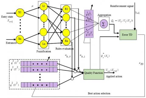
Figure 4 schematizes the structure of the apprentice proposed for the FQL algorithm in the case of discrete actions and continuous actions.
Figure 4. FQL in the case of discrete actions and continuous actions
3.2 FQL architecture for the optimization of conclusions
The architecture of the proposed FQL algorithm for the optimization of conclusions is shown in Figure 5.
The premise part of the SIF is fixed (all the states), the parameters of the conclusions, i.e., all the actions are available thanks to a priori knowledge of the system to be controlled, (27 actions for one 3-level inverter). The qualities of the actions are evaluated by the evaluation function Q [14, 15].
Consider a Takagi-Sugeno-type SIF, with initialization of identical conclusions for each fuzzy rule. A rule has the following form:
$\begin{aligned}
&R_{i}: \text { if } S_{1} \text { is } L_{1}^{i} \& \ldots \ldots . \& S_{N_{I}} \text { is } L_{N_{I}}^{i} \text { then } Y \text { is } a_{1} \text { with } q_{1}^{i}\\
&\begin{array}{l}
\text { or } a_{2} \text { with } q_{2}^{i} \\
\text { or } a_{3} \text { with } q_{3}^{i} \\
\quad \vdots \\
\text { or } a_{k} \text { with } q_{k}
\end{array}
\end{aligned}$ (9)
Figure 5. Architecture of the proposed FQL algorithm
And $i=1 \ldots N$
With,
- Ri the its basic rule;
- Y the output variable;
- $S=\left(S_{1}, \ldots \ldots \ldots, S_{N_{I}}\right)^{T}$ input variables whose domain of definition is denoted S;
- $L_{j}^{i}$ a linguistic term of the fuzzy variable used in the rule and whose membership function is noted $\mu_{L_{j}^{i}}$;
- {a1, a2, a3, a4, a5, …, ak} is the set of actions to be applied, it is either predefined from knowledge of the system to be controlled, or initialized randomly. It remains invariant during the learning process.
At the end of the learning process, the elected action Ae for each fuzzy rule is the action that has maximum quality.
At each time step. The SIF calculates the output action and the corresponding quality. This action is applied on the system which returns a reinforcement signal r. From this feedback signal, the quality value updated using the time difference method. An exploration / exploitation policy is implemented at the level of the FQL algorithm only at the start, thereafter it will be ensured by itself.
3.3 Procedure for executing the FQL algorithm
We describe the execution of the FQL algorithm over a time step. It can be divided into six main stages. Let t + 1 be the current time step, the apprentice applied the action (discrete or continuous) elected at the previous time step, and in return received the primary reinforcement due to the transition from state to state. He then perceives this state through the truth values of his rules and performs the following six steps:
(1). Calculation of the t-optimal evaluation function of the current state:
$Q_{t}^{*}\left(S_{t+1}\right)=\sum_{R_{i} \in A_{t}}\left(\operatorname{Max}_{U \in U}\left(q_{t}^{i}(U)\right) \alpha_{R_{i}}\left(S_{t+1}\right)\right.$ (10)
(2). Calculation of the TD error:
$\tilde{\varepsilon}_{t+1}=r_{t+1}+\gamma Q_{t}^{*}\left(S_{t+1}\right)-Q_{t}\left(S_{t}, U_{t}\right)$ (11)
(3). Update of the matrix:
$q_{t+1}^{i}=q_{t}^{i}+\beta \tilde{\varepsilon}_{t+1} e_{t}^{i^{T}}, \forall R_{i}$ (12)
(4). Election of the action applied on the state
• Discrete actions: inference of the overall quality of each discrete action from their local qualities:
$q_{t+1}^{S_{t+1}}(U)=q_{t+1}(U) \cdot \varphi_{t+1}^{T}, \forall U \in U,$ (13)
And election of one of these actions according to the exploration / exploitation policy:
$E_{U}\left(q_{t+1}^{S_{t+1}}\right)=A r g M a x_{U \in U}\left(q_{t+1}^{S_{t+1}}(U)+\eta^{S_{t+1}}(U)+\rho^{S_{t+1}}(U)\right)$ (14)
• Continuous actions: for each activated rule, election of a local action and inference of the continuous action to be applied:
$U_{t+1}\left(S_{t+1}\right)=\sum_{R_{i} \in A_{t+1}} E_{U}\left(q_{t+1}^{i}\right) \cdot \alpha_{R_{i}}\left(S_{t+1}\right), \forall U \in U$ (15)
where, election is defined by:
$E_{U}\left(q_{t+1}^{i}\right)=\operatorname{ArgMax}_{U \in U}\left(q_{t+1}^{i}(U)+\eta^{i}(U)+\rho^{i}(U)\right)$ (16)
5. Update of eligibility traces:
$e_{t+1}^{i}\left(U^{i}\right)=\left\{\begin{array}{l}
\gamma \lambda \cdot e_{t}^{i}\left(U^{i}\right)+\phi_{t+1}^{i},\left(U^{i}=U_{t+1}^{i}\right) \\
\gamma \lambda \cdot e_{t}^{i}\left(U^{i}\right), \quad \text { sinon }
\end{array}\right.$ (17)
6. New calculation of the evaluation function corresponding to the elected actions and the current state with the newly updated parameters:
$Q_{t+1}\left(S_{t+1}, U_{t+1}\right)=\sum_{R_{i} \in A_{t+1}} q_{t+1}^{i}\left(U_{t+1}^{i}\right) \alpha_{R_{i}}\left(S_{t+1}\right)$ (18)
This value will be used for the computation of the error TD at the next time step.
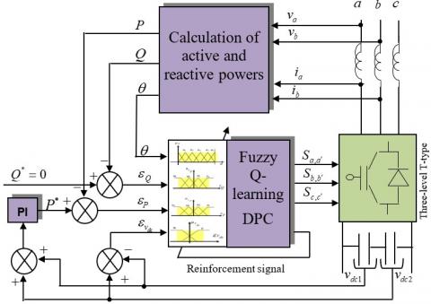
For analyzing the performance of the combining proposed algorithm, Figure 6 show the structure of chosen test system, which contain a three level T type converter, calculation unit and the implemented algorithm.
We validate the FQL algorithm applied to the settings of conclusions on DPC at three levels. Learning helps determine the best actions for each rule.
The definition of the point to be reached is carried out via four input variables: "reactive and active power errors", "angle error" and "the DC voltage error" respectively. The output variable is the possible actions "converter voltage vectors". We have chosen to use fuzzy logic reasoning to process these quantities.
Figure 6. Structure of studied system
4.1 The apprentice
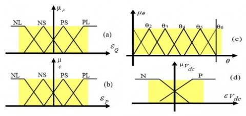
A Sugeno-type fuzzy controller has been used, where initially the conclusions Ai are all set to zero. The fuzzy controller inputs with four, six and two membership functions, respectively.
The fuzzy rules from which we have to find the conclusions are as follows:
If (active power error is Ai) and (reactive power error is Bj) and (DC voltage bus error is Ck) and (the angle is Dl) Then (Output is Vii) (1).
Or:
Ai is the fuzzy set of the active power error (2, 1, -1, -2) (i = 1:4).
Bj is the fuzzy set of the reactive power error (2, 1, -1, -2) (j= 1:4).
Bj is the fuzzy set of the reactive power error (2, 1, -1, -2) (j= 1:4).
Ck is the fuzzy set of the midpoint voltage error (1, -1) (k =1:2).
Dl is the fuzzy set where the "sector" voltage vector is located (l = 1:6).
Vii is the action elected in each rule from a set A of available actions (distinct vectors) (ii = 1:27).
The apprentice's task is to find the optimal actions for each fuzzy rule (Figure 7).
Figure 7. Fuzzy subsets of input variables
4.2 The reinforcement function
The reinforcement function used is defined as follows:
if (((active power _error) * (D_ active power _error) <0) & (reactive power _error) * (D_ reactive power _error) <0) & (DC voltage bus_error) * (D_ DC voltage bus _error) <0))) Then:
Ren = 10;
Else
Ren = -1;
End
The switching functions of each vector are represented as shown in Table 2:
Table 2. Switching tables with six angular sectors
|
ϴ1 |
|||||
|
Ԑ_P |
PL |
PS |
NS |
NL |
|
|
Ԑ_Q |
Ԑvdc |
||||
|
PL |
P |
V3 |
V16 |
V24 |
V11 |
|
N |
V3 |
V15 |
V23 |
V11 |
|
|
PS |
P |
V16 |
V16 |
V24 |
V24 |
|
N |
V15 |
V15 |
V23 |
V23 |
|
|
NS |
P |
V18 |
V18 |
V22 |
V22 |
|
N |
V17 |
V17 |
V21 |
V21 |
|
|
NL |
P |
V5 |
V18 |
V22 |
V9 |
|
N |
V5 |
V18 |
V21 |
V9 |
|
|
ϴ2 |
|||||
|
Ԑ_P |
PL |
PS |
NS |
NL |
|
|
Ԑ_Q |
Ԑvdc |
||||
|
PL |
P |
V5 |
V18 |
V14 |
V1 |
|
N |
V5 |
V17 |
V13 |
V1 |
|
|
PS |
P |
V18 |
V18 |
V14 |
V14 |
|
N |
V17 |
V17 |
V13 |
V13 |
|
|
NS |
P |
V20 |
V20 |
V24 |
V24 |
|
N |
V19 |
V19 |
V23 |
V23 |
|
|
NL |
P |
V7 |
V20 |
V24 |
V17 |
|
N |
V7 |
V19 |
V23 |
V11 |
|
|
ϴ3 |
|||||
|
Ԑ_P |
PL |
PS |
NS |
NL |
|
|
Ԑ_Q |
Ԑvdc |
||||
|
PL |
P |
V7 |
V20 |
V16 |
V3 |
|
N |
V7 |
V19 |
V15 |
V3 |
|
|
PS |
P |
V20 |
V20 |
V16 |
V16 |
|
N |
V19 |
V19 |
V15 |
V15 |
|
|
NS |
P |
V22 |
V22 |
V14 |
V14 |
|
N |
V21 |
V21 |
V13 |
V13 |
|
|
NL |
P |
V9 |
V22 |
V14 |
V1 |
|
N |
V9 |
V21 |
V13 |
V1 |
|
|
ϴ4 |
|||||
|
Ԑ_P |
PL |
PS |
NS |
NL |
|
|
Ԑ_Q |
Ԑvdc |
||||
|
PL |
P |
V9 |
V22 |
V18 |
V5 |
|
N |
V9 |
V21 |
V17 |
V5 |
|
|
PS |
P |
V22 |
V22 |
V18 |
V18 |
|
N |
V21 |
V21 |
V17 |
V17 |
|
|
NS |
P |
V24 |
V24 |
V16 |
V16 |
|
N |
V23 |
V23 |
V15 |
V15 |
|
|
NL |
P |
V11 |
V24 |
V16 |
V7 |
|
N |
V11 |
V23 |
V15 |
V7 |
|
|
ϴ5 |
|||||
|
Ԑ_P |
PL |
PS |
NS |
NL |
|
|
Ԑ_Q |
Ԑvdc |
||||
|
PL |
P |
V11 |
V24 |
V20 |
V7 |
|
N |
V11 |
V23 |
V19 |
V7 |
|
|
PS |
P |
V24 |
V24 |
V20 |
V20 |
|
N |
V23 |
V23 |
V19 |
V19 |
|
|
NS |
P |
V14 |
V14 |
V18 |
V18 |
|
N |
V13 |
V13 |
V17 |
V17 |
|
|
NL |
P |
V1 |
V14 |
V18 |
V5 |
|
N |
V1 |
V13 |
V17 |
V5 |
|
|
ϴ6 |
|||||
|
Ԑ_P |
PL |
PS |
NS |
NL |
|
|
Ԑ_Q |
Ԑvdc |
||||
|
PL |
P |
V1 |
V14 |
V22 |
V9 |
|
N |
V1 |
V13 |
V21 |
V9 |
|
|
PS |
P |
V14 |
V14 |
V22 |
V22 |
|
N |
V13 |
V13 |
V21 |
V21 |
|
|
NS |
P |
V16 |
V16 |
V20 |
V20 |
|
N |
V15 |
V15 |
V19 |
V19 |
|
|
NL |
P |
V3 |
V16 |
V20 |
V7 |
|
N |
V3 |
V15 |
V19 |
V7 |
|
For the studied system represented in Figure 6 above, the application of the proposed technic is illustrated by Figure 8 to 15 that represent the obtained results after simulation.
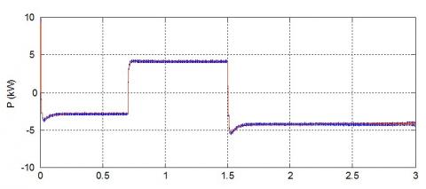
Note that the simulation was done using Matlab/SimPowerSystem environment and a fault was occurred at 0.7s and 1.5s designed by a change in desired reference of active power and at t=2.2s for reactive power.
First of all, Figures 8 and 9 show respectively, the active and reactive power in the AC side.
As showing in this result, the such active and reactive desired power mentioned by its references (red line), are perfectly obtained and they follow the references values, even when a change in refences happens (load variation for example), the VSC based on the FQL-DPC approach ensure this change in fraction of seconds and without any losses of response.
Figure 8. Active power
Figure 9. Reactive power
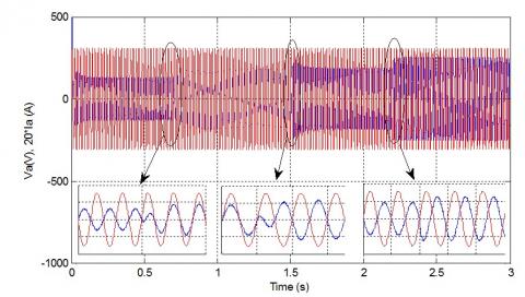
This response can be confirmed by evaluate the current and the voltage of the phases, that represented in Figure 10.
Taking phase (a) for the evaluation, we can see clearly that the VSC save it voltage in the desired reference, where the current change rapidly without losing it nature of signal, which is properly sinusoidal.
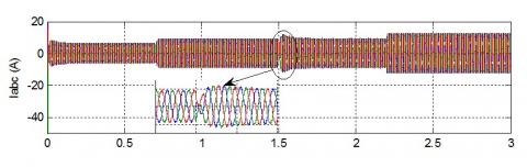
For better evaluation of the behaviour of the current, Figures 11, 12 and 13 shown the different current shift in the circuit.
From Figure 12, we can see the variation of current called by the load follow by a variation in the value of the current from -5A to 5A between 0.7s and 1.5s, in this period the behaviour of the current is slightly changed but it saves its sinusoidal shape (Figure 11).
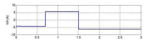
Also, the current in the middle point which name as Io showing in Figure 13 has variate with any change which confirm the reaction and the operation of the VSC base on Q learning DPC technique under any condition of working.
Figure 10. Voltage and current of phase a AC side
Figure 11. Three phase AC current
Figure 12. Load Current
Figure 13. Current zero in middle point
Figure 14. DC voltage of the DC side
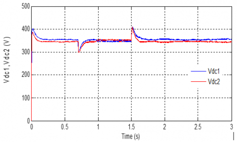
Figure 15. DC voltage of each capacity
Finally, in order to evaluate the characteristics of the control, we base on the response of the voltage on the DC side and the two capacitors builds the DC part of the VSC.
Figures 14 and 15 shown the response of the DC side, from these two figures, we can see the performance of the command adapted to control of the VSC.
At the transient period (reference variation), we can note exceedances of 11% with a response time of 1e-3s with a final value exactly the same (700V).
In the context offering a better control and ensure a good operation of a VSC, a new approach based on Fuzzy-Q-Learning algorithm and Direct Power Control is applied in this article.
Evaluating the obtained results after simulation, it’s appeared clearly that this technic enhances the response of VSC by maintaining its characteristics follow the reference values even the power side or the adopted command parameters.
The next work will be to combine this configuration on a real system such renewable source or FACTS devices.
|
AC |
Alternating current |
|
C1 |
Capacitor, F |
|
DC |
Direct current |
|
DPC |
Direct power control |
|
Dq |
Synchronous reference frame index |
|
FLC |
Fuzzy logic control |
|
FQL |
Fuzzy-Q-Learning |
|
irabc |
Line currents of the first network, A |
|
Lr |
Inductance, H |
|
P |
Power active, W |
|
Q |
Power reactive, var |
|
r |
Reinforcement signal |
|
Rr |
Resistance, Ω |
|
Vdck |
Voltage direct current (V) |
|
vrabc |
Simple voltages of the first network, V |
|
VSC |
Voltage source converter |
|
vtrabc |
Rectifier input voltages, V |
|
ωr |
Electrical pulsation of the grid |
[1] Nayak, N., Routray, S.K., Rout, P.K. (2014). Robust fuzzy sliding mode controller design for voltage source converter high-voltage DC based interconnected power system. Australian Journal of Electrical and Electronics Engineering, 11(4): 421-433. https://doi.org/10.7158/E13-203.2014.11.4
[2] Benchouia, N.E., Khochemane, L., Derghal, A., Madi, B., Mahmah, B., Aoul, E.H. (2015). An adaptive fuzzy logic control (AFLC) strategy for PEMFC fuel cell. International Journal of Hydrogen Energy, 40(39): 13806-13819. https://doi.org/10.1016/j.ijhydene.2015.05.189
[3] Berenji, H.R. (1994). Fuzzy Q-learning: A new approach for fuzzy dynamic programming. Proceedings of 1994 IEEE 3rd International Fuzzy Systems Conference, Orlando, FL, 1: 486-491. https://doi.org/10.1109/FUZZY.1994.343737
[4] Kofinas, P., Dounis, A.I., Vouros, G.A. (2018). Fuzzy Q-Learning for multi-agent decentralized energy management in microgrids. Applied Energy, 219: 53-67. https://doi.org/10.1016/j.apenergy.2018.03.017
[5] Zhang, Y.C., Qu, C.Q. (2015). Direct power control of a pulse width modulation rectifier using space vector modulation under unbalanced grid voltages. IEEE Transactions on Power Electronics, 30(10): 5892-5901. https://doi.org/10.1109/TPEL.2014.2371469
[6] Berkani, A., Negadi, K., Safa, A., Marignetti, F. (2020). Design and practical investigation of a model predictive control for power grid converter. TECNICA ITALIANA-Italian Journal of Engineering Science, 64(2-4): 354-360. https://doi.org/10.18280/ti-ijes.642-434
[7] Salem, A., Abido, M.A. (2019). T-Type multilevel converter topologies: A comprehensive review. Arab J Sci Eng, 44: 1713-1735. https://doi.org/10.1007/s13369-018-3506-6
[8] Stamer, F., Yüce, F., Singer, M., Hiller, M. (2018). Investigation of different balancing methods for modular 3-level T-type voltage source converters with distributed DC-link Capacitors. IECON 2018 - 44th Annual Conference of the IEEE Industrial Electronics Society, Washington, DC, pp. 1279-1284. https://doi.org/10.1109/IECON.2018.8592695
[9] Ngo, V.Q.B., Nguyen, M.K., Tran, T.T., Lim, Y.C., Choi, J.H. (2018). A simplified model predictive control for T-Type inverter with output LC filter. Energies, 12(1): 31. https://doi.org/10.3390/en12010031
[10] Schweizer, M., Kolar, J.W. (2012). Design and implementation of a highly efficient three-level T-type converter for low-voltage applications. IEEE Transactions on Power Electronics, 28(2): 899-907. https://doi.org/10.1109/TPEL.2012.2203151
[11] Xing, X.Y., Chen, A., Wang, W.S., Zhang, C.H., Li, Y.Z., Du, C.S. (2015). Space-vector-modulated for Z-source three-level T-type converter with neutral voltage balancing. 2015 IEEE Applied Power Electronics Conference and Exposition (APEC), Charlotte, NC, pp. 833-840, https://doi.org/10.1109/APEC.2015.7104446
[12] Berkani, A., Negadi, K., Allaoui, T., Marignetti, F. (2019). Generalized switching table of the DTC of an induction motor determined by reinforcement learning. U.P.B. Sci. Bull., Series C, 81(4): 205-218.
[13] Xu, M.L., Xu, W.B. (2010). Fuzzy Q-learning in continuous state and action space. The Journal of China Universities of Posts and Telecommunications, 17(4): 100-109. https://doi.org/10.1016/S1005-8885(09)60495-7
[14] Zajdel, R. (2010). Fuzzy Q(λ)-learning algorithm. In: Rutkowski L., Scherer R., Tadeusiewicz R., Zadeh L.A., Zurada J.M. (eds) Artificial Intelligence and Soft Computing. ICAISC 2010. Lecture Notes in Computer Science, vol 6113. Springer, Berlin, Heidelberg. https://doi.org/10.1007/978-3-642-13208-7_33
[15] Muñoz, P., Barco, R., de la Bandera, I. (2013). Optimization of load balancing using fuzzy Q-Learning for next generation wireless networks, Expert Systems with Applications, 40(4): 984-994. https://doi.org/10.1016/j.eswa.2012.08.071