Kang Li | Dan Li* | Daqing Wu
© 2020 IIETA. This article is published by IIETA and is licensed under the CC BY 4.0 license (http://creativecommons.org/licenses/by/4.0/).
OPEN ACCESS
With the improvement of enterprise services, location-routing-inventory problem with time window constraint (LRIPTW) has become an essential problem in cold chain logistics network (CCLN). This paper aims to optimize the location cost, inventory cost, transportation cost, and penalty cost in CCLN simultaneously. Firstly, an optimization model was established for the LRIP with soft time window constraint (STW). Then, the multi-objective ant colony optimization (MACO) was improved to solve the model. Simulation results show that the improved MACO can solve the LRIPSTW effectively and efficiently. The research findings provide a reference for enterprises to reduce total cost and improve service quality.
cold chain logistics network (CCLN), location-routing-inventory problem (LRIP), soft time window constraint (STW), multi-objective ant colony optimization (MACO)
Cold chain is a special supply chain with strict temperature requirements in the handling, holding, and transportation of products. Owing to the time-sensitivity of the quality of perishable products, it is important for cold chain logistics to meet the requirement on service time. To reduce supply chain cost, the cold chain logistics enterprise must satisfy the service time requirement by optimizing its location, routing, and inventory strategy. The service time can be divided into fuzzy time window (FTW), hard time window (HTW), and soft time window (STW).
Taking STW for example, every cold chain logistics enterprise must deliver the products in the STW required by customers. Early or late arrival will be penalized by customers according to the violation time, pushing up the total cost. To meet customer demand, perishable products need to be distributed within the prescribed time window constraint (TW). This helps to reduce the corruption rate of perishable products, and guarantee product quality.
This paper models the location-inventory-routing problem (LIRP) of cold chain logistics network (CCLN) under soft time window constraint (STW). In the model, customers have the right to penalize the cold chain logistics enterprise according to the length of violation time, forcing the enterprise to provide cold chain logistics services within the STW specified by customers.
Since the quality of perishable products declines with time, the corruption cost was considered to optimize the service cost. Then, the multi-objective ant colony optimization (MACO) was improved to solve the LIRPSTW. Simulation results show that the improved MACO can effectively minimize the total cost of the cold chain logistics enterprise in LIRPSTW.
The optimization of LRIPTW is a hot topic in supply chain management. Zarandi et al. [1] introduced FTW into location-routing problem (LRP), creating the LRPTW model which considers customer demand and FTW constraint under uncertain environment. Goncalves et al. [2] tackled vehicle routing problem with time window (VRPTW) and fuzzy customer demand, and solved the opportunity-constrained compensation model with a heuristic algorithm. Gong et al. [3] constructed a nonlinear integer programming model for the VRPTW, and developed a two-generation ant colony algorithm (ACA) to solve the problem. Saint-Guillain et al. [4] constructed a multi-objective dynamic programming model for dynamic VRP with TW and stochastic customers (DS-VRPTW), and solved the model with a novel global stochastic assessment (GSA) rule. Iqbal et al. [5] proposed the bee colony algorithm to solve the VRP with STW. Many scholars have noticed the difference between STW and HTW in solving the optimization model [6, 7]. Assuming that customers adopt (T, S) inventory strategy, Liu and Lee [8] presented the inventory-routing problem (IRP) with stochastic demand, constructed a mixed integer programming model for the problem with HTW, and solved the model through decomposition.
With the growing demand for perishable food, the optimization problems with TW has become a major concern in CCLN. Govindan et al. [9] proposed a multi-objective optimization model for a perishable food supply chain network (SCN), which aims to solve the two-echelon multiple-vehicle LRP with time-windows (2E-LRPTW) for sustainable SCN, and designed a novel multi-objective hybrid approach called MHPV to solve the model. Wei et al. [10-13] investigated an extension of IRP with route time limit in the cold chain, and developed a genetic algorithm (GA) to solve the formal mixed-integer linear program (MILP) model. Ma et al. [14-16] combined order selection and time-dependent vehicle routing problem with time windows into a new model for perishable product delivery, and solved the model with a hybrid ACA comprising local search operators. To maximize the profit of selling perishable products, Vahdani et al. [17] integrated production scheduling with VRP, and solved the integrated problem with two heuristic and meta-heuristic algorithms, thereby fulfilling customer satisfaction and the TW.
The research on the LRIPTW of CCLN generally focuses on a single or two problems, and transforms the LRIP into a single-objective problem. However, there is little report on the integrated multi-objectives LRIP with STW in CCLN. Compared with the existing literature, our research makes the following innovations: the impact of service time on cold chain logistics cost was thoroughly analysed; the STW was incorporated into the LRIP model of CCLN; the multi-objective problem was solved by an improved MACO. The research findings provide theoretical evidence and practical basis for cold chain logistics enterprise to improve service efficiency and customer satisfaction.
3.1 Problem description
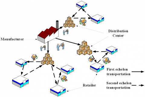
To meet the STW required by customers, the penalty cost was introduced to the LRIPSTW optimization model. As shown in Figure 1, the two-echelon CCLN consists of a manufacturer, several retailers, and multiple distribution centers (DCs).
Figure 1. The structure of the CCLN
This paper aims to fulfil three objectives: select the best DCs to minimize the location cost; determine the inventory quantity based on the quantity of ordered perishable products to minimize the inventory cost; optimize the distribution route to meet the STW of retailers to minimize the transportation cost and penalty cost.
3.2 Assumptions
(1) The CCLN has only one manufacturer, and each retailer is only served by on DC.
(2) The customer demand obeys random distribution.
(3) Each vehicle must leave from and return to the same DC, and serve only one retailer.
(4) All vehicles are of the same type with the same capacity.
(5) The loss of perishable products in the producing area is not considered.
(6) The temperature throughout the distribution process meets the quality and safety standards for perishable products.
(7) The corruption rate of perishable products remains constant.
(8) The penalty cost is imposed whenever a vehicle exceeds the STW.
3.3 Notations
(1) Sets
I is the set of DCs;
J is the set of retailers;
K is the set of vehicles.
(2) Parameters
Djis the annual demand of retailer J;
Qi is the order quantity of DCi;
fiis the fixed construction cost of DCi;
Oi is the cost for DCi to order products from the manufacturer;
hiis the unit inventory holding cost of DCi;
Liis the lead time of DCi;
α is the service level of DC;
P is the unit price of products;
θ is the corruption rate of products during transportation;
di is the travel distance from the manufacturer to DCi;
dgiis the travel distance from node (customer) g to node (customer) i;
pt is the transportation cost per unit distance of each product;
Viis the mean vehicle speed from the manufacturer to DCi;
Vgj is the mean vehicle speed from node g to node j;
Niis the maximum capacity of DCi;
b is the maximum capacity of each vehicle.
(3) Decision variables
Xi is the quantity of products transported the manufacturer to DCi;
Yij is the quantity of products transported from node i to node j;
$U_{i}=\left\{\begin{array}{cc}1 & \text { If } i \text { was chosen to be } \mathrm{DC} \\ 0 & \text { otherwise }\end{array} i \in I\right.$;
$R R_{i j}=\left\{\begin{array}{lc}1 & \text { If } \mathrm{DC}_{i} \text { serves retailer } J \\ 0 & \text { otherwise }\end{array} i \in I, j \in J\right.$;
$q_{g j k}=\left\{\begin{array}{lr}1 & \text { If vehicle travels from node } g \text { to node } j \\ 0 & \text { otherwise }\end{array}\right.$
$\forall g \in(I \cup J), \quad j \in J, k \in K$
3.4 Mathematical model
$\min {{Z}_{1}}=\sum\limits_{i\in I}^{{}}{{{f}_{i}}}{{U}_{i}}$ (1)
$\min {{Z}_{2}}={{p}_{t}}(\sum\limits_{i\in I}^{{}}{{{X}_{i}}}{{d}_{i}}{{U}_{i}}+\sum\limits_{k\in K}{\sum\limits_{g\in (I\bigcup J)}{\sum\limits_{j\in J}{{{Y}_{gj}}{{d}_{gj}}{{q}_{gjk}})+}}}p[\sum\limits_{i\in I}^{{}}{{{X}_{i}}}\left( 1-{{e}^{{-\theta {{d}_{i}}}/{{{v}_{i}}}\;}} \right)+\sum\limits_{k\in K}{\sum\limits_{g\in (I\bigcup J)}{\sum\limits_{j\in J}{{{Y}_{gj}}\left( 1-{{e}^{{-\theta {{d}_{gj}}}/{{{v}_{gj}}}\;}} \right){{q}_{gjk}}]}}}$ (2)
$\min Z_{3}=\sum_{i \in I}\left(O_{i} \sum_{j \in J} D_{j} R R_{i j} / Q_{i}+h_{i} Q_{i} / 2+h_{i} z_{\alpha_{0}} \sqrt{L_{i} \sum_{j \in J} \sigma_{j}^{2} R R_{i j}}\right)$ (3)
$\min Z_{4}=P_{d e} \sum_{j \in J} \max \left(E_{j}-T_{j k}, 0\right)+P_{d L} \sum_{j \in J} \max \left(T_{j k}-L_{j}, 0\right)$ (4)
Subject to:
$Q_{i}+z_{\alpha_{0}} \sqrt{L_{i} \sum_{j \in J} \sigma_{j}^{2} R R_{i j}} \leq N_{i}$ (5)
$\sum\limits_{j\in J}^{{}}{{{D}_{j}}}\sum\limits_{j\in J}^{{}}{{{q}_{gjk}}}\le b$ (6)
$\sum\limits_{k\in K}^{{}}{\sum\limits_{g\in (I\bigcup J)}^{{}}{{{q}_{gjk}}}}=1$ (7)
$\sum\limits_{j\in J}^{{}}{\sum\limits_{g\in (I\bigcup J)}^{{}}{{{q}_{gjk}}}}\le 1$ (8)
$\sum\limits_{k\in (I\bigcup J)}^{{}}{{{q}_{gjk}}}-\sum\limits_{k\in (I\bigcup J)}^{{}}{{{q}_{jgk}}}=0$ (9)
$\sum\limits_{i\in I}^{{}}{{{X}_{i}}}\ge \sum\limits_{j\in J}^{{}}{{{Y}_{ij}}}$ (10)
$\sum\limits_{i\in I}^{{}}{{{Y}_{ij}}}={{D}_{j}}$ (11)
${{T}_{jk}}=({{T}_{gk}}+S{{T}_{gk}}+{{d}_{gj}}/\text{ }{{V}_{gj}})\times {{q}_{gjk}}$,
$\forall g\in (I\bigcup J),j\in J,k\in K$ (12)
${{U}_{i}}=\left\{ 0,1 \right\},i\in I$ (13)
$R{{R}_{ij}}=\left\{ 0,1 \right\},i\in I,j\in J$ (14)
${{q}_{gjk}}=\left\{ 0,1 \right\},\forall g\in (I\bigcup J),j\in J$ (15)
Objective function (1) aims to minimize the location cost of DC in CCLN. Objective function (2) aims to minimize the transportation cost. Objective function (3) aims to minimize the inventory cost. Objective function (4) aims to minimize the penalty cost for the violation of the STW. Constraint (5) limits the capacity of each DC. Constraint (6) limits the capacity of each vehicle. Constraint (7) means each retailer is only served by one DC. Constraint (8) means each vehicle only serves one DC. Constraint (9) means no vehicle can remain on any node. Constraint (10) means the quantity of products transported to DCs is greater than that transported to the retailers. Constraint (11) means the demand of each retailer can be fulfilled. Constraint (12) means the arrival time of vehicle k at retailer j. Constraints (13)-(15) defines the possible values.
The LRIPSTW, as an extension of LRIP with capacity constraints, is non-deterministic polynomial-time (NP) hard. Heuristic algorithms can achieve good performance and results on such problems with a small number of computations. As a classical heuristic algorithm, ant colony optimization (ACO) is inspired by the foraging behavior of ant colonies. With excellence in solving combinatorial optimization problems in discrete space [18], the ACO has been widely adopted to solve traveling salesman problem (TSP), 0-1 knapsack, resource/vehicle scheduling problems [19-20].
The basic principle of the ACO is to simulate the foraging process of real ant colonies in nature: the ants in the same colony look for the optimal route by sharing special information to determine the distance and direction between them. However, slow convergence may occur if the ants have difficulty in finding the right route due to the lack of pheromones. Besides, the ACO might fall into the local optimum if the pheromone is not updated smoothly [21-23].
To overcome these defects, this paper improves the MACO with GA. To solve the LRIPSTW, the improved MACO incorporates the STW and product loss cost in ant state transition rules. The ant state transition rules, plus the uniformity of individual distribution, were improved to avoid the local optimum trap. In addition, the crossover operator A was introduced to diversify population distribution, enhancing the global search ability of the MACO.
4.1 MACO encoding
In the MACO, chromosomes are randomly generated as n-dimensional vectors [m1, m2, ..., mn], mi <{1, 2,..., n}, where miis retailer i. The optional DCs are numbered with 0. The vehicle load of each retailer is calculated when the vehicle leaves the DC 0. If the vehicle load exceeds the capacity constraint, the vehicle must return to DC 0. Then, the first sub-route will be generated. Starting from DC 0, the vehicle arrives at the next retailer, and repeats the above steps until the all retailers are served. Suppose there are 3 optional DCs and 6 retailers in the CCLN. The optional DCs are number from 1-3, and the retailers from 4-9, respectively. Figure 2 shows the chromosome generated from the CCLN. The three sub-routes are 0-6-4-0, 0-8-5-7-0, and 0-9-0.
Figure 2. An example of chromosome coding
In the improved MACO, DCs are selected for each sub-route by the following rules: (1) For each sub-route, the closest DCs to each retailer are computed separately; (2) The retailers are ranked by proximity to each DC; (3) The DC with the greatest number of closest retailers is selected. If all DC has the same number of closest retailers, the final DC is randomly chosen. By these rules, the final sub-routes are 2-6-4-2, 1-8-5-7-1, and 1-9-1.
4.2 State transition rules
The selection probability of each ant K moving from node i to node j can be expressed as:
$p_{k}(i, j)=\left\{\begin{array}{l}\frac{\left[\sum_{m=1}^{M} w_{m} \tau_{k}^{m}(i, j)\right]^{\alpha} \eta_{j}^{\beta}\left[\gamma_{j}\right]^{\varepsilon}\left[\omega_{j}\right]^{\lambda}}{\sum_{s \in L_{k}(i)}\left[\sum_{m=1}^{M} w_{m} \tau_{k}^{m}(i, j)\right]^{\alpha} \eta_{s}^{\beta}\left[\gamma_{s}\right]^{\varepsilon}\left[\omega_{s}\right]^{\lambda}}, q>q_{0} \\ \arg \max _{j \in L_{k}(i)}\left\{\left[\sum_{m=1}^{M} w_{m} \tau_{k}^{m}(i, j)\right]^{\alpha} \eta_{j}^{\beta}\left[\gamma_{j}\right]^{\varepsilon}\left[\omega_{j}\right]^{\lambda}\right\}, q \leq q_{0}\end{array}\right.$ (16)
where, γj is the time difference between the arrival time of vehicles from node i to node j and the upper limit of the STW; ε is the relative importance of the time difference; ωj is the waiting time of vehicles at node j; λ is the relative importance of the waiting time; q is a random variable uniformly distributed in [0, 1]; q0Î[0, 1] is a parameter that controls the transition rule. Under the state transition rules of the improved MACO, the node with relatively smaller time difference and short waiting time is highly likely to be selected.
4.3 Pheromone updating
When ant k selects node j from node i, the pheromone on edge (i, j) should be reduced to increase the probability of choosing other nodes. The local pheromone intensity can be updated by:
${{\tau }^{m}}(i,j)=(1-\zeta ){{\tau }^{m}}(i,j)+\zeta \vartriangle {{\tau }^{m}}(i,j)$ (17)
where $\zeta \in(0,1)$ is a constant; $(1-\zeta) \tau^{m}(i, j)$ is the volatilization of pheromones. Let Qm be the pheromones size (usually a constant), and fm be the value of the multi-objective function. After all ants complete a round of search, the global pheromone intensity can be updated by:
${{\tau }^{m}}(i,j)=(1-\rho ){{\tau }^{m}}(i,j)+\rho \vartriangle {{\tau }^{m}}(i,j)$ (18)
where, Gm is the pheromone size; min(fm) is the minimum value of the objective function m in the current Pareto frontier; $\Delta \tau^{m}(i, j)=\frac{G_{m}}{\min \left(f_{m}\right)}$. Then, the current solution is evaluated to update the Pareto frontier. If it is a non-dominant solution, the solution will be stored in the Pareto frontier; otherwise, the solution will be discarded.
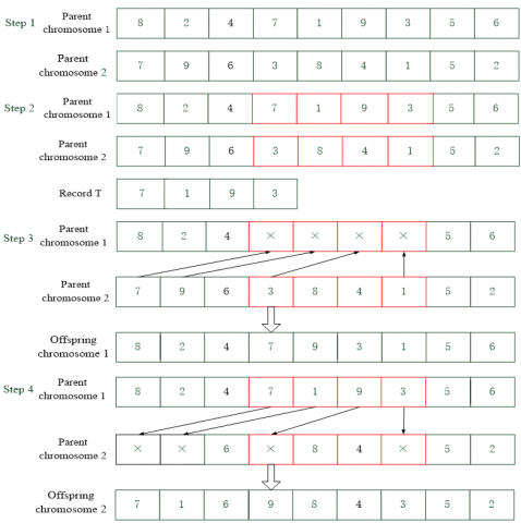
4.4 Crossover
Figure 3. An example of crossover operation
Based on the rules of the ACO, the crossover operator A was introduced to the improved MACO. To reduce the generation of illegal solution and improve the operation efficiency, this operator synthesizes the rules of traditional crossover operators like partial matched crossover (PMX), order crossover (OX), cycle crossover (CX) in the GA. The crossover operator A is generated in the following steps:
Step 1. Select two parent chromosomes 1 and 2 randomly.
Step 2. Select two cross points in parent chromosome 1 randomly, and save the part between the two points as a cross gene segment in the temporary record T.
Step 3. Identify and record the same gene in T from the other parent chromosome 2, and replace the vacant position in parent chromosome 1 with the same gene, producing offspring chromosome 1.
Step 4. Replace the vacant position in parent chromosome 2 with the gene segment recorded in T in sequence, producing offspring chromosome 2.
Figure 3 gives an example of crossover operation.
4.5 Mutation
Let p1Î(0,1) be the mutation probability. Then, a random number is generated between 0 and 1. If the random number is smaller than the mutation probability, the mutation operation will be executed. During the operation, two retailers are randomly selected from the CCLN. Then, the positions of the two retailers are swapped. Next, the new fitness values are calculated based on the optimization model. If the fitness values of the mutated chromosomes are better than those of the current chromosomes, the mutated ones will be retained.
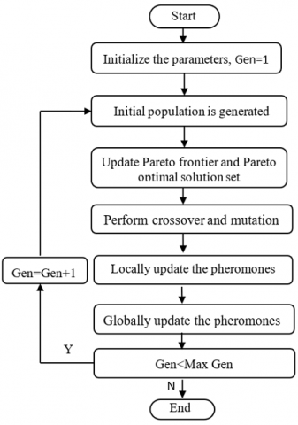
Figure 4. Flow chart of the improved MACO
The mutation of the improved MACO is implemented in the following steps:
Step 1. Initialize the parameters and place m ants on n optional DCs.
Step 2. Place the initial start point of each ant in the current solution set. Each ant K moves to the next retailer j at the probability calculated by formula (16). A chromosome is generated when each ant chooses all the nodes. The chromosomes produced by all the ants form the initial population.
Step 3. Calculate values of m objective functions for each ant, and update the Pareto frontier and Pareto optimal solution set.
Step 4. Perform crossover using the crossover operator A, followed by the mutation operation.
Step 5. Perform local update of pheromones by formula (17).
Step 6. Perform global update of pheromones by formula (18).
Step 7. If the number of iterations is smaller than the maximum number of iterations, return to Step 2.
Step 8. Terminate the algorithm.
Figure 4 illustrates the workflow of the improved MACO.
The improved MACO was verified through a simulation on a cold chain logistics enterprise for fresh agricultural products in Hangzhou, China. All the data were collected from the enterprise, and some parameter values were estimated based on the actual situation. The enterprise needs to select between three optional DCs to deliver perishable products to 18 supermarkets (retailers). The STWs required by the retailers are listed in Table 1.
The fixed construction costs of the DCs were generated randomly within [100, 200]. The penalty coefficient for time violation was set to 5. The setting of other relevant parameters is listed in Table 2. The parameters of the improved MACO were configured as α=1, β=5, ε=2, λ=3, ρ=0.1, ζ=100, and q0=0.7. The maximum number of iterations MAXGEN, crossover probability, and mutation probability were set to 150, 0.9, and 0.1, respectively.
Table 1. The STWs required by the retailers
|
Retailers |
4 |
5 |
6 |
7 |
8 |
9 |
|
STW |
(20,60] |
(15,55] |
(65,120] |
(50,100] |
(55,120] |
(60,120] |
|
Retailers |
10 |
11 |
12 |
13 |
14 |
15 |
|
STW |
(20,50] |
(25,60] |
(20,55] |
(65,100] |
(10,40] |
(15,55] |
|
Retailers |
16 |
17 |
18 |
19 |
20 |
21 |
|
STW |
(20,45] |
(50,105] |
(45,95] |
(18,50] |
(15,60] |
(55,96] |
Table 2. The parameter setting
|
Parameter |
Value |
Parameter |
Value |
|
σj2 |
20 |
P |
5yuan |
|
hi |
0.5yuan/kg |
Vi |
40km/h |
|
Oi |
20yuan per delivery |
Vgj |
40km/h |
|
Li |
7 |
pt |
0.03yuan/kg/km |
|
α0 |
97.5% |
Ni |
1,400kg |
|
θ |
0.05 |
b |
700kg |
The improved MACO was implemented in MATLAB R2014b and simulated on a laptop with Intel(R) Core (TM) i7-4610M 3.00GHz CPU, 8GB memory, and Windows 7 operating system. The simulation results are recorded in Table 3. As shown in Table 3, five routes were optimized when DCs 1, 2, and 3 were selected in turn. The penalty cost of the two routes from DC 3 was 126yuan, greater than that of any other routes. But their transportation cost was smaller than that of other routes. The two routes from DC 2 had a smaller penalty cost (65 yuan), yet a larger transportation cost than those from DC 3. Only one route starts from DC 1, whose penalty cost was 12yuan and transportation cost is 328yuan. In total, the cold chain logistics enterprise faced a location cost of 500yuan, an inventory cost of 331yuan, a transportation cost of 1,696yuan, a penalty cost of 212yuan, and a total cost of 2,739yuan.
Table 3. The simulation results
|
Selected DC |
Routes |
Location cost |
Inventory cost |
Transportation cost |
Penalty cost |
Total cost |
|
1 |
1-10-4-13-1 |
185 |
73 |
328 |
12 |
598 |
|
2 |
2-11-16-12-2 2-18-7-8-2 |
114 |
121 |
723 |
65 |
1023 |
|
3 |
3-20-19-14-21-3 3-17-9-15-5-3 |
201 |
137 |
645 |
135 |
1118 |
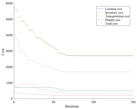
Figure 5. The cost change with the number of iterations
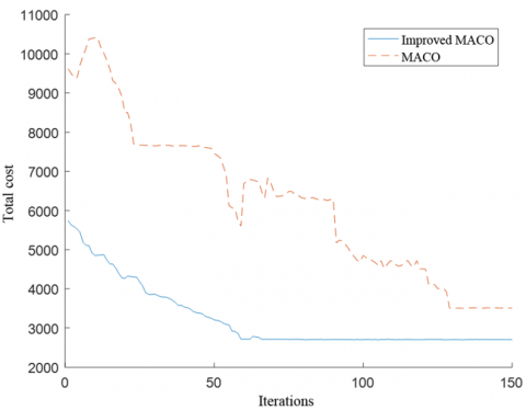
Figure 6. The comparison of convergence curves
Figure 5 displays the variations in the minimum values of location cost, inventory cost, transportation cost, penalty cost and the total cost with the number of iterations. It can be seen that every cost item of the enterprise continued to decrease with the growing number of iterations, which demonstrates the effectiveness of the improved MACO. The minimum values of location cost and inventory cost fluctuated greatly between the 5th and 30th iterations, suggesting that the improved MACO converges to the global optimal solution at the expense of an increase in an objective function. Any cost reduction will push up other costs. Therefore, there is no unique solution to the multi-objective problem, which optimizes different objectives simultaneously. Instead, a Pareto optimal solution set was formed for the LRIPSWT. The cold chain logistics enterprise can choose the best solution from the set based on the actual situation and requirements.
To verify its feasibility and effectiveness, the improved MACO was compared with the original MACO, using the same initial parameters. Figure 6 compares the convergence curves of the two algorithms. It can be seen that the improved MACO converged to the optimal solution in 62 iterations, while the original MACO converged in 130 iterations. Thus, the improved MACO clearly outperforms the original MACO in solving the LIRPSWT.
The paper proposes an LRIPSTW optimization model in CCLN, which considers the penalty cost of time violation. The model aims to optimize the location cost, inventory cost, transportation cost, and penalty cost simultaneously. Then, the original MACO was improved to solve the LRIPSTW optimization model. Specifically, the crossover operator A was introduced to diversify the population distribution and improve the global search ability; the ant state transition rules were improved to avoid the local optimum trap. Simulation results show that less violation of the STW can improve customer satisfaction at the expense of slightly increased transportation cost. Compared with the original MACO, the improved MACO can effectively optimize the LRIPSTW in CCLN.
This research was funded by the China education ministry humanities and social science research youth fund project (Grant No.: 18YJCZH192), the social science project in Hunan province (Grant No.: 16YBA316).
[1] Zarandi, M.H.F, Hemmati, A., Davari, S., Turksen, I.B. (2013). Capacitated location-routing problem with time windows under uncertainty. Knowledge-Based Systems, 37: 480-489. https://doi.org/10.1016/j.knosys.2012.09.007
[2] Goncalves, G., Hsu, T., Xu, J. (2009). Vehicle routing problem with time windows and fuzzy demands: an approach based on the possibility theory. International Journal of Advanced Operations Management, 1(4): 312-330. https://doi.org/10.1504/IJAOM.2009.031247
[3] Gong, W., Liu, X., Zhang J., Fu, Z.T. (2007). Two-generation ant colony system for vehicle routing problem with time windows. Wireless Communications, Networking and Mobile Computing 2007, International Conference on IEEE, pp. 1917-1920. https://doi.org/10.1109/WICOM.2007.480
[4] Saint-Guillain, M., Deville, Y., Solnon, C. (2015). A multistage stochastic programming approach to the dynamic and stochastic VRPTW. Integration of AI and or Techniques, 90(75): 357-374. https://doi.org/10.1007/978-3-319-18008-3_25
[5] Iqbal, S., Kaykobad, M., Rahman, M.S. (2015). Solving the multi-objective vehicle routing problem with soft time windows with the help of bees. Swarm and Evolutionary Computation, 24: 50-64. https://doi.org/10.1016/j.swevo.2015.06.001
[6] Shi, W., Weise, T. (2013). An initialized ACO for the VRPTW. Intelligent Data Engineering and Automated Learning, 82(6): 93-100. https://doi.org/10.1007/978-3-642-41278-3_12
[7] Balseiro, S.R., Loiseau, I., Ramonet, J. (2011). An ant colony algorithm hybridized with insertion heuristics for the time dependent vehicle routing problem with time windows. Omr and Oraon Rarh, 38(6): 954-966. https://doi.org/10.1016/j.cor.2010.10.011
[8] Liu, S.C., Lee, W.T. (2011). A heuristic method for inventory routing problem with time windows. Expert Systems with Applications, 38: 13223-13231. https://doi.org/10.1016/j.eswa.2011.04.138
[9] Govindan, K., Jafarian, A., Khodaverdi, R., Devika, K. (2014). Two-echelon multiple-vehicle location–routing problem with time windows for optimization of sustainable supply chain network of perishable food. International Journal of Production Economics, 152: 9-28. https://doi.org/10.1016/j.ijpe.2013.12.028
[10] Wei, C., Gao, W.W., Hu, Z.H., Yin, Y.Q., Pan, S.D. (2019). Assigning customer-dependent travel time limits to routes in a cold-chain inventory routing problem. Computers & Industrial Engineering, 133: 275-291. https://doi.org/10.1016/j.cie.2019.05.018
[11] Li, J., Zhang, L.Y., Feng, X.J., Jia, K.K., Kong, F.B. (2019). Feature extraction and area identification of wireless channel in mobile communication. Journal of Internet Technology, 20(2): 545-553. https://doi.org/10.3966/160792642019032002021.
[12] Fu, H.L., Manogaran, G., Wu, K., Cao, M., Jiang, S., Yang, A. (2019). Intelligent decision-making of online shopping behavior based on Internet of Things. International Journal of Information Management, 50: 515-525. https://doi.org/10.1016/j.ijinfomgt.2019.03.010.
[13] Yang, A.M., Zhang, C.Y., Chen, Y.J., Zhuansun, Y.X., Liu, H.X. (2019). Security and privacy of smart home systems based on the Internet of Things and Stereo Matching Algorithms. IEEE Internet of Things Journal, 7(4): 2521-2530. https://doi.org/10.1109/JIOT.2019.2946214
[14] Ma, Z.J., Wu, Y., Dai, Y. (2017). A combined order selection and time-dependent vehicle routing problem with time widows for perishable product delivery. Computers & Industrial Engineering, 114: 101-113. https://doi.org/10.1016/j.cie.2017.10.010
[15] Yang, A.M., Zhuansun, Y.X., Liu, C.S., Li, J., Zhang C. (2019). Design of intrusion detection system for internet of things based on improved BP neural network. IEEE Access, 7: 106043-106052. https://doi.org/10.1109/ACCESS.2019.2929919
[16] Mi, C., Shen, Y., Mi, W.J., Huang, Y. (2015). Ship identification algorithm based on 3D point cloud for automated ship loaders. Journal of Coastal Research, 73(sp1): 28-34. https://doi.org/10.2112/si73-006.1
[17] Vahdani, B., Niaki, S.T.A., Aslanzade, S. (2017). Production-inventory-routing coordination with capacity and time window constraints for perishable products: Heuristic and meta-heuristic algorithms. Journal of Cleaner Production, 161(10): 598-618.
[18] Coello, C., De Computación, S., Zacatenco, C. Twenty years of evolutionary multi-objective optimization: A historical view of the field. IEEE Computational Intelligence Magazine, 1(1): 28-36. https://doi.org/10.1109/mci.2006.1597059
[19] Mavrovouniotis, M., Müller, F.M., Yang, S.X. (2017). Ant colony optimization with local search for dynamic traveling salesman problems. IEEE Transactions on Cybernetics, 47(1): 1743-1756. https://doi.org/10.1109/TCYB.2016.2556742
[20] Zajac, P. (2011). The idea of the model of evaluation of logistics warehouse systems with taking their energy consumption under consideration. Archives of Civil and Mechanical Engineering, 11(2): 479-492. https://doi.org/10.1016/S1644-9665(12)60157-5
[21] Goudarzi, F., Asgari, H., Al-Raweshidy H.S. (2019). Traffic-aware VANET routing for city environments-a protocol based on ant colony optimization. IEEE Systems Journal, 13(1): 571-581.
[22] Butanda, J.A., Málaga, C., Plaza, R.G. (2017). On the stabilizing effect of chemotaxis on bacterial aggregation patterns. Applied Mathematics & Nonlinear Sciences, 2(1): 157-172. https://doi.org/10.21042/AMNS.2017.1.00013
[23] Sudhakar, S., Francis, S., Balaji, V. (2017). Odd mean labeling for two star graph. Applied Mathematics & Nonlinear Sciences, 2(1): 195-200. https://doi.org/10.21042/AMNS.2017.1.00016