Abdallah Lemita | Sebti Boulahbel | Sami Kahla* | Moussa Sedraoui
© 2020 IIETA. This article is published by IIETA and is licensed under the CC BY 4.0 license (http://creativecommons.org/licenses/by/4.0/).
OPEN ACCESS
Dissolved oxygen (DO) concentration is a key variable in the activated sludge wastewater treatment processes. In this paper, an auto control strategy based on Euler method and gradient method with radial basis function (RBF) neural networks (NNs) is proposed to solve the DO concentration control problem in an activated sludge process of wastewater treatment. The control purpose is to maintain the dissolved oxygen concentration in the aerated tank for having the substrate concentration within the standard limits established by legislation of wastewater treatment. For that reason, a new proposed control strategy based on gradient descent method and RBF neural network has been used. Compared with RBF neural network PI control, the obtained results show the effectiveness in terms of both transient and steady performances of proposed control method for dissolved oxygen control in the activated sludge wastewater treatment processes.
activated sludge process, wastewater treatment, gradient descent algorithm, RBF neural network, PI control
The wastewater treatment process is a very complex process; it presents strong nonlinearity and uncertainties regarding to its parameters. The wastewater treatment comprises various steps used for reducing the contaminants in the wastewater which are: pretreatment, primary treatment, secondary treatment [1, 2]. The pretreatment has the objective of removing solid objects, and to skimming off floating greases and oils. Without passing the wastewater through the pretreatment, these objects may cause block and damage the equipment and the other steps of treatments. The primary treatment removes the remaining suspended and dissolved solids.
The secondary or biological treatment is the most important step of wastewater treatment. It aims to add microorganisms to reduce the organic matter, nitrogen and phosphorus from the wastewater. There are different methods used in the wastewater treatment process, but the most used and popular one is the activated sludge process (ASP) [3, 4].
In the last years, varieties of researches have been conducted about the control of the level of dissolved oxygen to enhance the process. In general, improvements are related to the controlling techniques. A linear proportional integral (PI) controller with feedforward from the flow rate and the respiration rate has been shown as a basic strategy [4]. Because of the PID controller limitation, the classical method of proportional integral derivative (PID) has been attempted, and the controlling effect of the dissolved oxygen is not satisfactory enough. However, the controllers are normally designed for the particular operational conditions because of the scarcity of sufficient hard or soft sensors and the nonlinear features of the bioprocesses [5]. In recent times, scholars have begun to study the artificial intelligence (AI) technologies which can be widely implemented in numerous areas, including chemical and biochemical processes and. Due to its great capabilities and adaptabilities of nonlinear modelling, the most prevalent AI controlling strategies are neural network and fuzzy network, which are usually integrated with the PID control. A fuzzy method to the control of dissolved oxygen in the process of aeration was studied by Man et al. [6]. An adaptive fuzzy control strategy for dissolved oxygen concentration was used to control of an activated sludge process Liu et al. [7]. In the paper [8] an adaptive fuzzy neural network-based model predictive control (AFNN-MPC) is proposed for the control problem of DO concentration. Piotrowski proposed a supervisory heuristic fuzzy control system applied to a Sequencing Batch Reactor (SBR) in the Wastewater Treatment Plant (WWTP) [9]. Lin and Luo [10] developed an adaptive neural technique using a disturbance observer to solve the dissolved oxygen concentration control problem. An improved multi objective optimal control (MOOC) strategy is developed to improve the operational efficiency, satisfy the effluent quality (EQ) and reduce the energy consumption (EC) in wastewater treatment process [11]. Mirghasemi proposed a robust adaptive neural network control strategy and used it to control the dissolved oxygen in activated sludge process application [12].
In this paper, a control strategy based on Euler method and gradient method with RBF neural network is proposed to control the dissolved oxygen concentration in an activated sludge process of wastewater treatment. The Euler is a numerical method that is used to approximate the solution of a nonlinear differential equation (nonlinear system), and the gradient descent algorithm and the RBF neural network are used to find the values of a function's parameters (coefficients) that minimize a performance function as possible. The performance of the proposed control strategies laws is illustrated with numerical simulations comparing their results with RBFNN-PI controller.
The remainder of this paper is organized as follows: in Section 2, Euler method is clearly discussed, in Section 3, presents a nonlinear control strategy based on gradient method accompanied with neural network method. In Section 4, RBF neural network PI control is discussed. The Section 5, a mathematical model of wastewater treatment process is given. In Section 6, the simulation results are presented. Finally, it is ended by a conclusion.
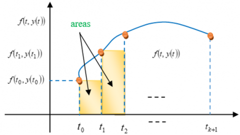
The Euler's method is numerical method that is used to approximate the solutions of a differential equation (Figure 1). Let consider the following differential equation:
$\frac{\partial y\left( t \right)}{\partial t}=f\left( t,y\left( t \right) \right)$ (1)
$\forall t\in \Re ,y\left( 0 \right)={{y}_{0}}$ is the initial condition.
t: time variable, y: output system.
The principal of Euler's method is to integrate the two parts of Eq. (1) between t0 and t1.
$\int\limits_{{{t}_{0}}}^{{{t}_{1}}}{\frac{\partial y\left( t \right)}{\partial t}}dt=\int\limits_{{{t}_{0}}}^{{{t}_{1}}}{f\left( t,y\left( t \right) \right)dt}$ (2)
$y\left( {{t}_{1}} \right)=y\left( {{t}_{0}} \right)+\int\limits_{{{t}_{0}}}^{{{t}_{1}}}{f\left( t,y\left( t \right) \right)dt}$ (3)
The integral $\int\limits_{{{t}_{0}}}^{{{t}_{1}}}{f\left( t,y\left( t \right) \right)dt}$ can be approximated by:
* The area of upper rectangle of $f\left( {{t}_{0}},y\left( {{t}_{0}} \right) \right)$ and length${{t}_{1}}-{{t}_{0}}=h$. Then:
$\int\limits_{{{t}_{0}}}^{{{t}_{1}}}{f\left( t,y\left( t \right) \right)dt\approx h.f\left( {{t}_{0}},y\left( {{t}_{0}} \right) \right)}$ (4)
Figure 1. Euler method
* The area of upper rectangle of $f\left( {{t}_{1}},y\left( {{t}_{1}} \right) \right)$ and length ${{t}_{1}}-{{t}_{0}}=h$. Then:
$\int\limits_{{{t}_{0}}}^{{{t}_{1}}}{f\left( t,y\left( t \right) \right)dt\approx h.f\left( {{t}_{1}},y\left( {{t}_{1}} \right) \right)}$ (5)
* The following statement results from the application of the trapezoidal rule in the approximation integration of the integral in Eq. (2).
$\int\limits_{{{t}_{0}}}^{{{t}_{1}}}{f\left( t,y\left( t \right) \right)dt\approx \frac{h}{2}.\left( f\left( {{t}_{0}},y\left( {{t}_{0}} \right) \right)+f\left( {{t}_{1}},y\left( {{t}_{1}} \right) \right) \right)}$ (6)
By using Eq. (4), The numerical solution of Eq. (1) can be given by the following equation:
$y\left( {{t}_{1}} \right)=y\left( {{t}_{0}} \right)+h.f\left( {{t}_{0}},y\left( {{t}_{0}} \right) \right)$ (7)
For $k\ge 0$:
$y\left( {{t}_{k+1}} \right)=y\left( {{t}_{k}} \right)+h.f\left( {{t}_{k}},y\left( {{t}_{k}} \right) \right)$ (8)
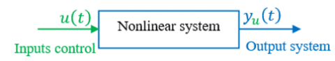
Now, consider a nonlinear system that can be written as the following differential equation:
$\frac{\partial {{y}_{u}}\left( t \right)}{\partial t}=f\left( t,{{y}_{u}}\left( t \right),u\left( t \right) \right)$ (9)
Figure 2. Nonlinear system with single input-single output
The curve of the output system ${{y}_{u}}\left( {{t}_{k}} \right)$ depends on the input control u(t). If we consider two different inputs control u(t)=u0, and u(t)=u1, then Eq. (9) yields:
$\frac{\partial {{y}_{{{u}_{0}}}}\left( t \right)}{\partial t}=f\left( t,{{y}_{{{u}_{0}}}}\left( t \right),{{u}_{0}} \right)$ (10)
$\frac{\partial {{y}_{{{u}_{1}}}}\left( t \right)}{\partial t}=f\left( t,{{y}_{{{u}_{1}}}}\left( t \right),{{u}_{1}} \right)$ (11)
The numerical solutions of these equations (Eq. (10) and Eq. (11)) by using Euler's method are:
${{y}_{{{u}_{0}}}}\left( {{t}_{k+1}} \right)={{y}_{{{u}_{0}}}}\left( {{t}_{k}} \right)+h.f\left( {{t}_{k}},{{y}_{{{u}_{0}}}}\left( {{t}_{k}} \right),{{u}_{0}} \right)$ (12)
${{y}_{{{u}_{1}}}}\left( {{t}_{k+1}} \right)={{y}_{{{u}_{1}}}}\left( {{t}_{k}} \right)+h.f\left( {{t}_{k}},{{y}_{{{u}_{1}}}}\left( {{t}_{k}} \right),{{u}_{1}} \right)$ (13)
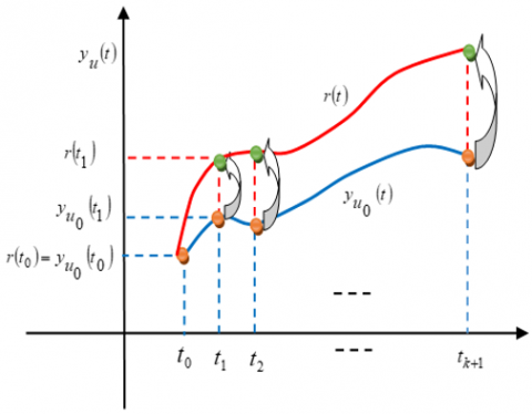
Figure 3 shows the curves of Eq. (12) and Eq. (13).
Figure 3 shows that if we apply two different inputs u(t)=u0 and u(t)=u1 on system in Figure 2, we will have two different trajectories in the output system. Suppose that we know the input u(t)=u0, if we want that the trajectory ${{y}_{{{u}_{0}}}}\left( {{t}_{k+1}} \right)$ (blue curve) tracks the trajectory ${{y}_{{{u}_{1}}}}\left( {{t}_{k+1}} \right)$ (red curve), we have to find the value of input control u1 that makes the trajectory ${{y}_{{{u}_{0}}}}$tracks the trajectory ${{y}_{{{u}_{1}}}}$.
The aim of the proposed control strategy is to control the system output ${{y}_{{{u}_{0}}}}\left( {{t}_{k+1}} \right)$ to track a desired reference $r\left( {{t}_{k+1}} \right)$by changing at every instant tk the value of input control uk.
Figure 3. Curve of Eq. (9) with two different inputs control $u\left( t \right)={{u}_{0}}$ and $u\left( t \right)={{u}_{1}}$
The proposed control strategy is depicted in Figure 4.
Figure 4. Curve of Principal of the proposed control strategy
Consider the following nonlinear system:
$\frac{\partial {{y}_{{{u}_{0}}}}\left( t \right)}{\partial t}=f\left( t,{{y}_{{{u}_{0}}}}\left( t \right),{{u}_{0}} \right)$ (14)
The numerical solution of Eq. (14) by using Euler's method is:
${{y}_{{{u}_{0}}}}\left( {{t}_{1}} \right)={{y}_{{{u}_{0}}}}\left( {{t}_{0}} \right)+h.f\left( {{t}_{0}},{{y}_{{{u}_{0}}}}\left( {{t}_{0}} \right),{{u}_{0}} \right)$ (15)
At time t1, we have to find the value of the input control u1 to get: ${{y}_{{{u}_{0}}}}\left( {{t}_{1}} \right)=r\left( {{t}_{1}} \right)$.
${{y}_{{{u}_{1}}}}\left( {{t}_{1}} \right)={{y}_{{{u}_{0}}}}\left( {{t}_{0}} \right)+h.f\left( {{t}_{0}},{{y}_{{{u}_{0}}}}\left( {{t}_{0}} \right),{{u}_{1}} \right)$ (16)
The input control u1 is adjusted by using the gradient descent algorithm by minimizing the performance function with respect to u0.The performance function is the squared error $E({{t}_{1}})$ between ${{y}_{{{u}_{1}}}}({{t}_{1}})$ and ${{y}_{{{u}_{0}}}}({{t}_{1}})$.
$E\left( {{t}_{1}} \right)=\frac{1}{2}{{\left( e\left( {{t}_{1}} \right) \right)}^{2}}=\frac{1}{2}{{\left( {{y}_{{{u}_{1}}}}\left( {{t}_{1}} \right)-{{y}_{{{u}_{0}}}}\left( {{t}_{1}} \right) \right)}^{2}}$ (17)
$E\left( {{t}_{1}} \right)=\frac{1}{2}{{\left( r\left( {{t}_{1}} \right)-{{y}_{{{u}_{0}}}}\left( {{t}_{1}} \right) \right)}^{2}}$ (18)
Input control u1 updating by using the gradient descent algorithm:
${{u}_{1}}={{u}_{0}}+\Delta {{u}_{0}}$ (19)
$\Delta {{u}_{0}}=-\lambda .\frac{\partial E\left( {{t}_{1}} \right)}{\partial {{u}_{0}}}$ (20)
Then:
${{u}_{1}}={{u}_{0}}-\lambda .\frac{\partial E\left( {{t}_{1}} \right)}{\partial {{u}_{0}}}$ (21)
where, $\lambda $: learning rate.
${{u}_{1}}={{u}_{0}}-\lambda .\frac{\partial E\left( {{t}_{1}} \right)}{\partial {{y}_{{{u}_{0}}}}\left( {{t}_{1}} \right)}.\frac{\partial {{y}_{{{u}_{0}}}}\left( {{t}_{1}} \right)}{\partial f\left( {{t}_{0}},{{y}_{{{u}_{0}}}}\left( {{t}_{0}} \right),{{u}_{0}} \right)}.\frac{\partial f\left( {{t}_{0}},{{y}_{{{u}_{0}}}}\left( {{t}_{0}} \right),{{u}_{0}} \right)}{\partial {{u}_{0}}}$ (22)
${{u}_{1}}={{u}_{0}}+\lambda .e\left( {{t}_{1}} \right).h.\frac{\partial f\left( {{t}_{0}},{{y}_{{{u}_{0}}}}\left( {{t}_{0}} \right),{{u}_{0}} \right)}{\partial {{u}_{0}}}$ (23)
${{u}_{1}}={{u}_{0}}+\lambda .e\left( {{t}_{1}} \right).\frac{\partial {{y}_{{{u}_{0}}}}\left( {{t}_{1}} \right)}{\partial {{u}_{0}}}$ (24)
In general case, it is difficult to calculate the expression of $\frac{\partial {{y}_{{{u}_{0}}}}\left( {{t}_{1}} \right)}{\partial {{u}_{0}}}$ , therefore, it has been known that the neural network can approximate any nonlinear function, then, it can be used to approximate $\frac{\partial {{y}_{{{u}_{0}}}}\left( {{t}_{1}} \right)}{\partial {{u}_{0}}}$.
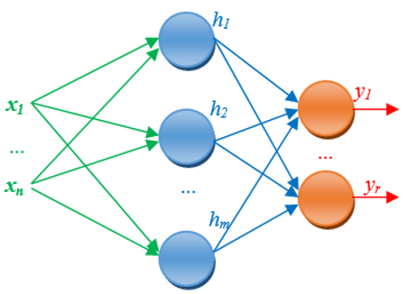
3.1 RBF neural network algorithm
Figure 5. RBF neural network structure
A radial basis function neural network (RBFNN) is introduced into neural network in the paper [13], it has three layers: an input layer, a nonlinear hidden layer that uses Gaussian function as activation function, and a linear output layer [14]. The RBF networks have many uses, including function approximation, classification, and system control. It has the advantage of fast learning speed and is able to avoid the problem of local minimum.
The structure of the RBF neural network is illustrated in Figure 5.
The output of the ${{j}^{th}}$ hidden neurons is given by the following equation:
${{h}_{j}}=\exp \left( -\frac{{{\left\| X-{{C}_{i,j}} \right\|}^{2}}}{2b_{j}^{2}} \right)$ (25)
where, $X=\left[x_{1}, x_{2}, \ldots, x_{n}\right]^{T}$ is the input vector of the neural network.
The RBF neural network output is described in the following equation:
${{y}_{RBFNN}}=\sum\nolimits_{j=1}^{m}{{{W}_{l,j}}{{h}_{j}}}=\sum\nolimits_{j=1}^{m}{{{W}_{l,j}}}\exp \left( -\frac{{{\left\| X-{{C}_{i,j}} \right\|}^{2}}}{2b_{j}^{2}} \right)$ (26)
where, Wl,j is the weight between the hidden layer and the output layer. The center Ci,j, the basis width parameter bj and the weights Wl,j of the RBF neuron network are adjusted by using the gradient descent algorithm to minimize the sum of square error ERBFNN.
The expression of ERBFNN is given as follow:
${{E}_{RBFNN}}=\frac{1}{2}{{\sum\nolimits_{{}}^{{}}{\left( {{e}_{RBFNN}}\left( k \right) \right)}}^{2}}=\frac{1}{2}{{\sum\nolimits_{k=1}^{r}{\left( {{y}_{{{u}_{k}}}}\left( k \right)-{{y}_{RBFNN}}\left( k \right) \right)}}^{2}}$ (27)
${{C}_{i,j}}\left( k \right)={{C}_{i,j}}\left( k-1 \right)+\Delta {{C}_{i,j}}+\alpha \left( {{C}_{i,j}}\left( k-1 \right)-{{C}_{i,j}}\left( k-2 \right) \right)$ (28)
${{b}_{j}}\left( k \right)={{b}_{j}}\left( k-1 \right)+\Delta {{b}_{j}}+\alpha \left( {{b}_{j}}\left( k-1 \right)-{{b}_{j}}\left( k-2 \right) \right)$ (29)
${{W}_{l,j}}\left( k \right)={{W}_{l,j}}\left( k-1 \right)+\Delta {{W}_{l,j}}+\alpha \left( {{W}_{l,j}}\left( k-1 \right)-{{W}_{l,j}}\left( k-2 \right) \right)$ (30)
The corresponding modifier formulas are as follows:
$\Delta {{C}_{i,j}}=-\eta \frac{\partial {{E}_{RBFNN}}}{\partial {{C}_{i,j}}}=-\eta \frac{\partial {{E}_{RBFNN}}}{\partial {{y}_{RBFNN}}}\frac{\partial {{y}_{RBFNN}}}{\partial {{h}_{j}}}\frac{\partial {{h}_{j}}}{\partial {{C}_{i,j}}}$ (31)
$\Delta {{C}_{i,j}}=\eta .{{e}_{RBF}}{{W}_{l,j}}{{h}_{j}}.\left( \frac{X-{{C}_{i,j}}}{b_{j}^{2}} \right)$ (32)
$\Delta {{b}_{j}}=-\eta \frac{\partial {{E}_{RBFNN}}}{\partial {{b}_{j}}}=-\eta \frac{\partial {{E}_{RBFNN}}}{\partial {{y}_{RBFNN}}}\frac{\partial {{y}_{RBFNN}}}{\partial {{h}_{j}}}\frac{\partial {{h}_{j}}}{\partial {{b}_{j}}}$ (33)
$\Delta {{b}_{j}}=\eta .{{e}_{RBFNN}}{{W}_{l,j}}{{h}_{j}}.\frac{{{\left\| X-{{C}_{i,j}} \right\|}^{2}}}{b_{j}^{3}}$ (34)
$\Delta {{W}_{l,j}}=-\eta \frac{\partial {{E}_{RBFNN}}}{\partial {{W}_{l,j}}}=-\eta \frac{\partial {{E}_{RBFNN}}}{\partial {{y}_{RBFNN}}}\frac{\partial {{y}_{RBFNN}}}{\partial {{W}_{l,j}}}$ (35)
$\Delta {{W}_{l,j}}=\eta .{{e}_{RBFNN}}.{{h}_{j}}$ (36)
where, a is the momentum factor, and h is the learning rate.
From Eq. (24), we have:
${{u}_{1}}={{u}_{0}}+\lambda .e\left( {{t}_{1}} \right).\frac{\partial {{y}_{{{u}_{0}}}}\left( {{t}_{1}} \right)}{\partial {{u}_{0}}}$ (37)
The RBF neural network will be used to calculate the expression of $\frac{\partial {{y}_{{{u}_{0}}}}\left( {{t}_{1}} \right)}{\partial {{u}_{0}}}$.
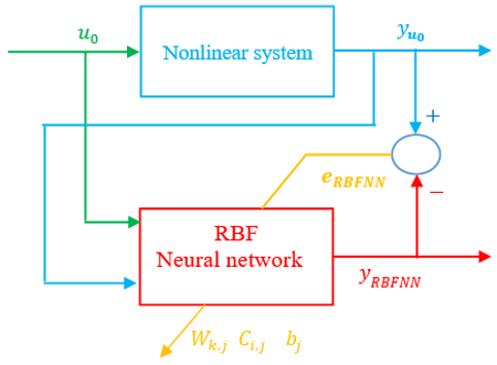
The schema of RBF neural network identification is depicted in Figure 6.
Figure 6. Schema of RBF neural network identification
If the RBF neural network output yRBFNN is equal to the system output ${{y}_{{{u}_{0}}}}$ [15, 16], then, we can use the expression of yRBFNN to calculate the expression of $\frac{\partial {{y}_{{{u}_{0}}}}\left( {{t}_{1}} \right)}{\partial {{u}_{0}}}$.
$\frac{\partial {{y}_{{{u}_{0}}}}\left( {{t}_{1}} \right)}{\partial {{u}_{0}}}\approx \frac{\partial {{y}_{RBFNN}}}{\partial {{u}_{0}}}=\frac{\partial }{\partial {{u}_{0}}}\sum\nolimits_{j=1}^{r}{{{W}_{1,j}}}{{h}_{j}}$ (38)
$\frac{\partial {{y}_{{{u}_{0}}}}\left( {{t}_{1}} \right)}{\partial {{u}_{0}}}=\frac{\partial }{\partial {{u}_{0}}}\sum\nolimits_{j=1}^{r}{{{W}_{1,j}}}\exp \left( -\frac{{{\left\| X-{{C}_{i,j}} \right\|}^{2}}}{2b_{j}^{2}} \right)$ (39)
$\frac{\partial {{y}_{{{u}_{0}}}}\left( {{t}_{1}} \right)}{\partial {{u}_{0}}}=\sum\nolimits_{j=1}^{r}{{{W}_{1,j}}\frac{\partial }{\partial {{u}_{0}}}}\exp \left( -\frac{{{\left\| X-{{C}_{i,j}} \right\|}^{2}}}{2b_{j}^{2}} \right)$ (40)
$\begin{align} & \frac{\partial {{y}_{{{u}_{0}}}}\left( {{t}_{1}} \right)}{\partial {{u}_{0}}}=\sum\nolimits_{j=1}^{r}{{{W}_{1,j}}\frac{\partial }{\partial {{x}_{1}}}} \\ & \exp \left( -\frac{{{X}^{T}}X-{{X}^{T}}{{C}_{i,j}}-C_{i,j}^{T}X+C_{i,j}^{T}{{C}_{i,j}}}{2b_{j}^{2}} \right) \\ \end{align}$ (41)
With: $X={{\left[ \begin{matrix} {{u}_{0}} & {{y}_{{{u}_{0}}}} \\\end{matrix} \right]}^{T}}={{\left[ \begin{matrix} {{x}_{1}} & {{x}_{2}} \\\end{matrix} \right]}^{T}}$
${{C}_{i,j}}=\left[ \begin{matrix} {{C}_{1,1}} & \begin{matrix} {{C}_{1,2}} & ... & {{C}_{1,m}} \\\end{matrix} \\ {{C}_{2,1}} & \begin{matrix} {{C}_{2,2}} & ... & {{C}_{2,m}} \\\end{matrix} \\\end{matrix} \right]$
$\begin{align} & \frac{\partial {{y}_{{{u}_{0}}}}\left( {{t}_{1}} \right)}{\partial {{u}_{0}}}=\sum\nolimits_{j=1}^{r}{{{W}_{1,j}}\frac{\partial }{\partial {{x}_{1}}}}\exp \\ & \left( -\frac{\left[ \begin{matrix} {{x}_{1}} & {{x}_{2}} \\\end{matrix} \right]\left[ \begin{matrix} {{x}_{1}} \\ {{x}_{2}} \\\end{matrix} \right]-\left[ \begin{matrix} {{x}_{1}} & {{x}_{2}} \\\end{matrix} \right].{{C}_{i,j}}-C_{i,j}^{T}\left[ \begin{matrix} {{x}_{1}} \\ {{x}_{2}} \\\end{matrix} \right]+C_{i,j}^{T}{{C}_{i,j}}}{2b_{j}^{2}} \right) \\ \end{align}$ (42)
$\begin{align} & \frac{\partial {{y}_{{{u}_{0}}}}\left( {{t}_{1}} \right)}{\partial {{u}_{0}}}=\sum\nolimits_{j=1}^{r}{{{W}_{1,j}}\frac{\partial }{\partial {{x}_{1}}}}\exp \\ & \left( -\frac{x_{1}^{2}+x_{2}^{2}-2{{x}_{1}}{{C}_{1,j}}-2{{x}_{2}}C_{2,j}^{T}+C_{i,j}^{T}{{C}_{i,j}}}{2b_{j}^{2}} \right) \\ \end{align}$ (43)
$\begin{align} & \frac{\partial {{y}_{{{u}_{0}}}}\left( {{t}_{1}} \right)}{\partial {{u}_{0}}}=\sum\nolimits_{j=1}^{r}{{{W}_{1,j}}\left( \frac{{{C}_{1,j}}-{{x}_{1}}}{b_{j}^{2}} \right)}.\exp \\ & \left( -\frac{x_{1}^{2}+x_{2}^{2}-2{{x}_{1}}{{C}_{1,j}}-2{{x}_{2}}C_{2,j}^{T}+C_{i,j}^{T}{{C}_{i,j}}}{2b_{j}^{2}} \right) \\ \end{align}$ (44)
So:
$\frac{\partial {{y}_{{{u}_{0}}}}\left( {{t}_{1}} \right)}{\partial {{u}_{0}}}=\sum\nolimits_{j=1}^{r}{{{W}_{1,j}}\left( \frac{{{C}_{1,j}}-{{x}_{1}}}{b_{j}^{2}} \right)}.{{h}_{j}}$ (45)
We substitute Eq. (45) in Eq. (37) to get the control law:
${{u}_{1}}={{u}_{0}}+\lambda .e\left( {{t}_{1}} \right).\sum\nolimits_{j=1}^{r}{{{W}_{1,j}}\left( \frac{{{C}_{1,j}}-{{x}_{1}}}{b_{j}^{2}} \right)}.{{h}_{j}}$ (46)
The steps of the proposed control strategy are as follows:
Step1. We start by u=u0 (the choice of u0 depend on the study system).
Step2. Initializing the network parameters: the number of nodes in input, hidden and output layer, the center Ci,j, the basis width parameter bj and the weights Wl,j, learning rate.
Step3. for k³0.
- Calculating the output ${{y}_{{{u}_{k}}}}\left( {{t}_{k+1}} \right)$ and network output yRBFNN(tk+1), calculating the error eRBFNN(tk+1).
- Adjusting of neural network parameters: Ci,j, bj and Wl,j from Eq. (32), Eq. (34) and Eq. (36).
- Calculating error e(tk+1) between ${{y}_{{{u}_{k}}}}\left( {{t}_{k+1}} \right)$ and r(tk+1).
- Calculating the new value of uk+1 via the following expression:
${{u}_{k+1}}={{u}_{k}}+\lambda .e\left( {{t}_{k+1}} \right).\sum\nolimits_{j=1}^{r}{{{W}_{1,j}}\left( \frac{{{C}_{1,j}}-{{u}_{k}}}{b_{j}^{2}} \right)}.{{h}_{j}}$ (47)
Step 4. We replace the found value of uk+1 on the system.
${{y}_{{{u}_{0}}}}\left( {{t}_{k+1}} \right)={{y}_{{{u}_{0}}}}\left( {{t}_{k}} \right)+h.f\left( {{t}_{k}},{{y}_{{{u}_{0}}}}\left( {{t}_{k}} \right),{{u}_{k+1}} \right)$ (48)
According to this algorithm, we can obtain: ${{y}_{{{u}_{0}}}}\left( {{t}_{k+1}} \right)=r\left( {{t}_{k+1}} \right)$.
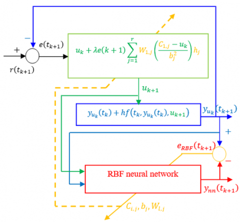
The structure of the proposed method is illustrated in Figure 7.
Figure 7. Schema of the proposed control strategy
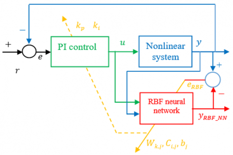
Figure 8. Adaptive RBF neural network PI structure
The structure of the RBF neural network PI is based on two control strategy (Figure 8), the first one is a conventional PI control because of its good control performance and the second is the RBF neural network control strategy. The PI control is used for controlling the dissolved oxygen concentration in the aerobic reactor, and the RBF neural network is used to regulate the parameters of PI control: kp and ki for improving the adaptability of the controller.
The mathematical expression of the PI (Proportional Integral) control algorithm is given by the following equation:
$u\left( k \right)=u\left( k-1 \right)+{{k}_{p}}\left( e\left( k \right)-e\left( k-1 \right) \right)+{{k}_{i}}e\left( k \right)$ (49)
where, u(k) is the output of the PI control (the input control of the system) and e is the error between the desired output r and actual system output.
$e\left( k \right)=r\left( k \right)-y\left( k \right)$ (50)
It has been known that the PI control performance is based on the value of PI parameters kp and ki. To improve the performance of the PI controller against the disturbance on the system, the parameters kp and ki can be auto-adjusted and optimized, so, the adaptive PI control algorithm became:
$u\left( k \right)=u\left( k-1 \right)+{{k}_{p}}\left( k \right)\left( e\left( k \right)-e\left( k-1 \right) \right)+{{k}_{i}}\left( k \right)e\left( k \right)$ (51)
The parameters of PI controller (kp and ki) are adjusted (auto-tuning) by using the gradient descent algorithm to minimize the sum of squared error E between the system output y and the desired output r.
The performance function E is defined as:
$E{{\left( k \right)}_{{}}}=\frac{1}{2}{{\sum\nolimits_{k=1}^{N}{\left( r\left( k \right)-y\left( k \right) \right)}}^{2}}=\frac{1}{2}{{\sum\nolimits_{k=1}^{N}{\left( e\left( k \right) \right)}}^{2}}$ (52)
According to the gradient descent method, the adjustment rules of the PI parameters are given as:
${{k}_{p}}\left( k \right)={{k}_{p}}\left( k-1 \right)+\Delta {{k}_{p}}$ (53)
${{k}_{i}}\left( k \right)={{k}_{i}}\left( k-1 \right)+\Delta {{k}_{i}}$ (54)
where,
$\Delta {{k}_{p}}=-\eta \frac{\partial E}{\partial {{k}_{p}}}=-\eta \frac{\partial E}{\partial y}\frac{\partial y}{\partial u}\frac{\partial u}{\partial {{k}_{p}}}=\eta e\left( k \right)\frac{\partial y}{\partial u}\left( e\left( k \right)-e\left( k-1 \right) \right)$ (55)
$\Delta {{k}_{i}}=-\eta \frac{\partial E}{\partial {{k}_{i}}}=-\eta \frac{\partial E}{\partial y}\frac{\partial y}{\partial u}\frac{\partial u}{\partial {{k}_{i}}}=\eta e\left( k \right)\frac{\partial y}{\partial u}e\left( k \right)$ (56)
where,
$\frac{\partial y}{\partial u}=\sum\nolimits_{j=1}^{r}{{{W}_{1,j}}\left( \frac{{{C}_{1,j}}-{{x}_{1}}}{b_{j}^{2}} \right)}.{{h}_{j}}$ (57)
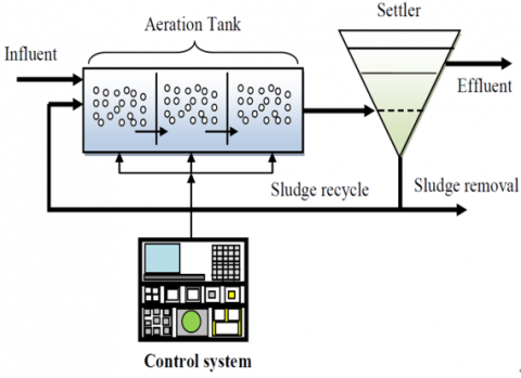
The schematic of the wastewater treatment process is represented in Figure 9.
Figure 9. Schema of activated sludge process
The aeration tank is a biological reactor in which the microorganisms are developed by removing the organic substrate in the presence of the dissolved oxygen concentration. In the settler tank the solids are separated from the wastewater. The growth of micro-organisms (biomass) in the aeration tank is not sufficient, then, a part of the removed sludge (the sludge contains the biomass) is recycled back tothe aeration tank while the other part is removed from the system.
The mathematical model considered in this paper contains four differential equations, the biomass concentrationX, the substrate concentration S, the dissolved oxygen concentration DO and the recycled biomass concentration Xr. The model is given by the following equations [17, 18].
$\frac{\partial X\left( t \right)}{\partial t}=\mu \left( t \right).X\left( t \right)-D.\left( 1+r \right).X\left( t \right)+r.D.{{X}_{r}}\left( t \right)$ (58)
$\frac{\partial S\left( t \right)}{\partial t}=-\frac{1}{Y}\mu \left( t \right).X\left( t \right)-D.\left( 1+r \right).S\left( t \right)+D.{{S}_{in}}$ (59)
$\frac{\partial DO\left( t \right)}{\partial t}=-\frac{{{K}_{0}}}{Y}\mu \left( t \right).X\left( t \right)-D.\left( 1+r \right).DO\left( t \right)+KLa.\left( D{{O}_{\max }}-DO\left( t \right) \right)+D.D{{O}_{in}}$ (60)
$\frac{\partial {{X}_{r}}\left( t \right)}{\partial t}=D.\left( 1+r \right).X\left( t \right)-D.\left( \beta +r \right).{{X}_{r}}\left( t \right)$ (61)
With:
$\mu \left( t \right)={{\mu }_{\max }}.\frac{S\left( t \right)}{S\left( t \right)+{{k}_{s}}}.\frac{DO\left( t \right)}{DO\left( t \right)+{{k}_{DO}}}$ (62)
$KLa=\alpha .W\left( k \right)$.
W: the aeration flow rate.
The aeration rate W is considered in this paper as the variable control for controlling the oxygen concentration in the aeration tank. Table 2 and Table 3 below show the parameters and initial values of the model respectively.
Table 2. Model parameters
|
Description |
Parameters |
Units |
Values |
|
Biomass yield factor |
Yh |
- |
0.65 |
|
Maximum specific growth rate |
mmax |
h-1 |
0.15 |
|
Half-saturation coefficient for micro-organisms |
ks |
mg. l-1 |
100 |
|
Oxygen half-saturation coefficient for micro-organisms |
kDO |
mg. l-1 |
2 |
|
Maximum DO concentration |
DOmax |
mg. l-1 |
10 |
|
Model constant |
K0 |
- |
0.5 |
|
Oxygen transfer rate |
a |
- |
0.018 |
|
Ratio of recycled |
r |
- |
0.6 |
|
Ratio of waste flow |
b |
- |
0.2 |
|
Influent substrate concentration |
Sin |
mg. l-1 |
200 |
|
Influent DO concentration |
DOin |
mg. l-1 |
0.5 |
|
Oxygen mass transfer coefficient |
KLa |
h-1 |
- |
|
Aeration rate |
W |
m3. h-1 |
- |
|
Dilution rate |
D |
${{h}^{-1}}$ |
- |
Table 3. Initial values
|
Variables concentrations |
Symbols |
Units |
Values |
|
Substrate concentration |
Ss |
mg. l-1 |
88 |
|
Biomass concentration |
X |
mg. l-1 |
20 |
|
Dissolved oxygen concentration |
DO |
mg. l-1 |
2 |
|
Recycle biomass concentration |
Xr |
mg. l-1 |
320 |
This paper proposes a control strategy based on Euler and gradient method based on Radial basis function neural network (RBFNN) is used to control the organic substances concentration in the aeration tank through the control of the dissolved oxygen concentration.
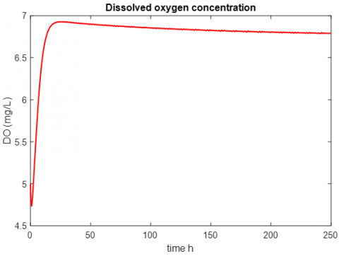
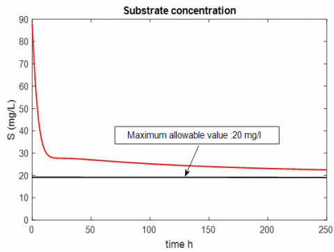
Figures 10 and 11 show the dissolved oxygen and substrate concentration in open loop (no control technique is applied to control the dissolved oxygen concentration). We can see clearly that the substrate concentration exceeds the maximum allowable value 20mg.l-1, so, the control of the dissolved oxygen concentration became obligatory for having a substrate concentration below the standard limit.
Figure 10. Dissolved oxygen concentration
Figure 11. Substrate concentration
For comparison, RBF neural network PI controller has been used with the initial’s parameters: kp=3 and ki=0.9.
The RBF neural network has the following structure (for the proposed control strategy and RB neural network PI control): two inputs in input layer X=[W DO]T, six neurons in hidden layer, and one neuron in output layer. The RBF neural network parameters Ci,j, bj and Wk,j are respectively initialized in the range [30, 60], [20, 40], and [0, 10], the learning rate m=0.09 and he momentum factor a=0.5.
The step size h=0.5.
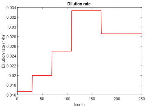
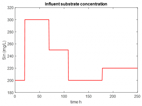
The dilution rate (Figure 12) is considered variable to cover many different regimes: high flow D=0.035h-1, normal flow D=0.025h-1 and low flow D=0.015h-1. The influent substrate concentration Sin is also considered with different values to assure a real study of wastewater system (Figure 13).
Figure 12. Dilution rate
Figure 13. Influent substrate concentration
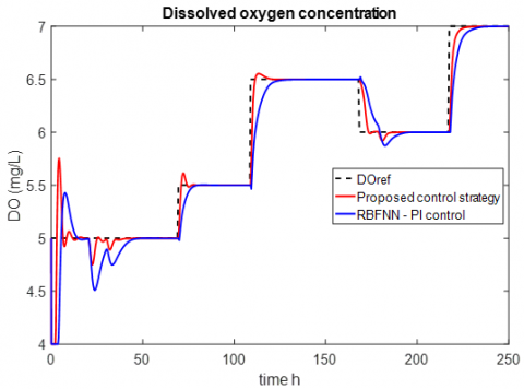
Figure 14. Dissolved oxygen concentration with modified dilution rate and influent substrate
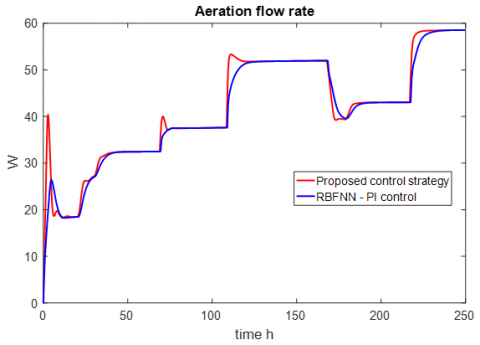
From Figure 14, when the dilution rate and the influent substrate concentration changed, the RBFNN-PI controller is very affected by these changes and it is not well tracking the set-point reference DOref, contrary of the proposed method that is not very affected by these disturbances generated by dilution rate and the influent substrate concentration. The dissolved oxygen concentration has a good tracking of the set-point reference DOref by using the proposed control strategy. The aeration rate (control variable) is depicted in Figure 15.
Figure 16, shows clearly that substrate concentration is biologically degraded below the maximum allowable value 20mg.l-1.
Figure 15. Aeration rate (Control variable)
Figure 16. Substrate concentration
The criterions IAE (integral of absolute error) and ISE (integral of square error) are used to compare the performance of the different control strategies:
$IAE=\int\limits_{0}^{\infty }{\left| e\left( t \right) \right|}dt$ (63)
$ISE=\int\limits_{0}^{\infty }{e{{\left( t \right)}^{2}}}dt$ (64)
The simulations results are compared from the view point of integral of absolute error (IAE). Considering this measure, the dissolved oxygen concentration has the best results applying the proposed controller (Table 1).
Table 1. Simulated IAE and ISE of the controllers
|
Used control methods |
IAE |
ISE |
|
RBFNN-PI controller |
0.1232 |
0.0740 |
|
Proposed controller |
0.0678 |
0.0455 |
In this paper, an Euler control strategy and gradient method based on RBFNN has been established to control the substrate concentration via the control of the dissolved oxygen concentration in an activated sludge process of wastewater treatment. The effectiveness of the proposed method was evaluated through a comparison with RBF neural network PI controller. The simulation results indicate that the proposed control strategy has a better performance for tracking the set-point reference DOref compared to the RBF neural network PI control.
[1] Babuponnusami, A., Muthukumar, K. (2014). A review on Fenton and improvements to the Fenton process for wastewater treatment. Journal of Environmental Chemical Engineering, 2(1): 557-572. https://doi.org/10.1016/j.scitotenv.2019.03.180
[2] Passos, F., Gutiérrez, R., Brockmann, D., Steyer, J.P., García, J., Ferrer, I. (2015). Microalgae production in wastewater treatment systems, anaerobic digestion and modelling using ADM1. Algal Research, 10: 55-63. https://doi.org/10.1016/j.algal.2015.04.008
[3] Mannina, G., Ekama, G., Caniani, D., Cosenza, A., Esposito, G., Gori, R., Olsson, G. (2016). Greenhouse gases from wastewater treatment-A review of modelling tools. Science of the Total Environment, 551: 254-270. https://doi.org/10.1016/j.scitotenv.2016.01.163
[4] Du, X., Wang, J., Jegatheesan, V., Shi, G. (2018). Dissolved oxygen control in activated sludge process using a neural network-based adaptive PID algorithm. Applied Sciences, 8(2): 261. https://doi.org/10.3390/app8020261
[5] Holenda, B., Domokos, E., Rédey, Á., Fazakas, J. (2008). Dissolved oxygen control of the activated sludge wastewater treatment process using model predictive control. Computers & Chemical Engineering, 32(6): 1270-1278. https://doi.org/10.1016/j.compchemeng.2007.06.008
[6] Man, Y., Shen, W., Chen, X., Long, Z., Corriou, J.P. (2018). Dissolved oxygen control strategies for the industrial sequencing batch reactor of the wastewater treatment process in the papermaking industry. Environmental Science: Water Research & Technology, 4(5): 654-662. https://doi.org/10.1039/C8EW00035B
[7] Liu, D., Zong, X. (2019). Dissolved oxygen control in sewage treatment process based on fuzzy active disturbance rejection control. In 2019 IEEE 3rd Advanced Information Management, Communicates, Electronic and Automation Control Conference (IMCEC), pp. 1164-1168. https://doi.org/10.1109/IMCEC46724.2019.8983931
[8] Han, H., Liu, Z., Qiao, J. (2019). Fuzzy neural network-based model predictive control for dissolved oxygen concentration of WWTPs. International Journal of Fuzzy Systems, 21: 1497-1510. https://doi.org/10.1007/s40815-019-00644-8
[9] Piotrowski, R. (2020). Supervisory fuzzy control system for biological processes in sequencing wastewater batch reactor. Urban Water Journal, 17(4): 325-332. https://doi.org/10.1080/1573062X.2020.1778744
[10] Lin, M.J., Luo, F. (2016). Adaptive neural control of the dissolved oxygen concentration in WWTPs based on disturbance observer. Neurocomputing, 185: 133-141. https://doi.org/10.1016/j.neucom.2015.12.045
[11] Han, H.G., Zhang, L., Liu, H.X., Qiao, J.F. (2018). Multiobjective design of fuzzy neural network controller for wastewater treatment process. Applied Soft Computing, 67: 467-478. https://doi.org/10.1016/j.asoc.2018.03.020
[12] Mirghasemi, S., Macnab, C.J.B., Chu, A. (2014). Dissolved oxygen control of activated sludge bioreactors using neural-adaptive control. In Proceedings of the IEEE Symposium on Computational Intelligence in Control and Automation (CICA 2014), Orlando, FL, USA, pp. 9-12. https://doi.org/10.1109/CICA.2014.7013237
[13] Macnab, C.J.B. (2014). Stable neural-adaptive control of activated sludge bioreactors. In Proceedings of the 2014 American Control Conference (ACC2014), Portland, OR, USA, pp. 4-6. https://doi.org/10.1109/ACC.2014.6858627
[14] Qiao, J.F., Hou, Y., Zhang, L., Han, H.G. (2018). Adaptive fuzzy neural network control of wastewater treatment process with multiobjective operation. Neurocomputing, 275: 383-393. https://doi.org/10.1016/j.neucom.2017.08.059
[15] Han, H.G., Qiao, J.F., Chen, Q.L. (2012). Model predictive control of dissolved oxygen concentration based on a self-organizing RBF neural network. Control Engineering Practice, 20(4): 465-476. https://doi.org/10.1016/j.conengprac.2012.01.001
[16] Ruan, J., Zhang, C., Li, Y., Li, P., Yang, Z., Chen, X., Huang, M., Zhang, T. (2017). Improving the efficiency of dissolved oxygen control using an on-line control system based on a genetic algorithm evolving FWNN software sensor. Journal of Environmental Management, 187: 550-559. https://doi.org/10.1016/j.jenvman.2016.10.056
[17] Belchior, C.A.C., Araújo, R.A.M., Landeck, J.A.C. (2012). Dissolved oxygen control of the activated sludge wastewater treatment process using stable adaptive fuzzy control. Computers & Chemical Engineering, 37: 152-162. https://doi.org/10.1016/j.compchemeng.2011.09.011
[18] Jeppsson, U., Rosen, C., Alex, J., Copp, J., Gernaey, K.V., Pons, M.N., Vanrolleghem, P.A. (2006). Towards a benchmark simulation model for plant-wide control strategy performance evaluation of WWTPs. Water Sci. Technol, 53(1): 287-295. https://doi.org/10.2166/wst.2006.031