Ying Wang* | Zongzhong Tian
© 2020 IIETA. This article is published by IIETA and is licensed under the CC BY 4.0 license (http://creativecommons.org/licenses/by/4.0/).
OPEN ACCESS
This paper proposes an efficient origin-estimation bandwidth (OD band) model, which provides dedicated progression bands for arterial traffic based on the real-time dynamic matrix of their estimated OD pairs. The innovations of the OD band model are as follows: First, the dynamics of through and turning-in/out traffics are analyzed based on the matrix of their estimated OD pairs, and used to generate the traffic movement sequence at continuous intersections; Second, the end-time of green interval for lag-lag phase sequence at continuous intersections is determined according to the relevant constraints, the relationship between the start/end-time of green interval and the minimum/maximum green intervals; Third, the bandwidths of the two directions of the artery ware produced, after being weighted by their traffic demands. The intuitiveness, convenience, and feasibility of the OD band model were fully demonstrated through a case study. Overall, the OD band model helps to produce bi-directional progression bands for traffic with many turning movements on the artery, and enables the through and turning-in/out traffics to proceed through continuous intersections, when the signals at those intersections are green.
arterial network, traffic signal coordination (TSC), movement sequence, minimum/maximum green intervals, progression bands
Traffic signal coordination (TSC), which is essential to the operation of arterial network, has long attracted the attention of the academia. The most famous TSC approaches are based on bandwidth and disutility. The bandwidth-based approaches have gained more popularity than disutility-based ones thanks to their high visuality [1]. Maximum bandwidth [2] and multiple bandwidth [3] are two fundamental bandwidth-based approaches. For convenience, the two approaches are referred to as maxband and multiband, respectively.
Proposed by Morgan and Little in 1964, maxband was extended two years later using a mixed-integer formulation, and generalized as a computation program in 1981 [4]. As a symmetric, uniform-width bandwidth system, maxband provides a feasible solution to the bi-directional bandwidth for arterial TSC: the total bandwidth of the artery is apportioned as per the directional volume ratio of the entire artery, under the guidance of progression design. However, maxband has two prominent defects: First, the arterial TSC performance is dampened by the neglection of the turning-in and turning-out traffic at each intersection [5, 6]; second, the band end-time cannot be changed by the advanced queue clearance time that serves the turning-in traffic arriving at the target intersection in the red interval from the upstream.
In 1991, Gartner et al. extended maxband into multiband, which derives a variable bandwidth from the multiple bands/weights of bi-directional road sections. This bandwidth system is symmetric, variable-width in each direction, and asymmetric between the two directions. The bandwidth varies with the directional weights in the overall objective function. Despite its superiority over maxband in supply and demand, multiband overlooks the dynamics of traffic movements. For instance, the turning-in traffic, which increases the through traffic, arrives at the through lanes of the target intersection before the through traffic from the upstream; meanwhile, the turning-out traffic, which reduces the through traffic, is randomly distributed in the traffic flow. The multiband cannot change the band end-time, because the through traffic from the upstream always arrive at a fixed time. Based on the volume and offset of turning-in traffic, Chen et al. [7] improved the queue clearance time in maxband into a variable queue clearance time model, yet failed to take account of the overall bandwidth.
In recent years, evident progress has been made on arterial TSC. Zhang et al. [8] modified multiband into an asymmetric multiband model, which generates asymmetric progression bands with varying widths for different segments of the artery, and improves the use of available green intervals. Taking the queue clearance time as cross-bands, Arsava et al. [9] improved maxband into origin-destination bandwidth (OD band) model, in which the bandwidths are weighted by the number of segments traversed by the turning-in traffic from the sides and by the traffic volume. Hu et al. [10] replaced mix-integer linear programming of arterial TSC with a mathematical optimization model. Based on real-time dynamic OD matrix, Ding et al. [11] developed an arterial TSC method in the light of turning-in/out movements. Nevertheless, the above arterial TSC strategies give no consideration to the movements of actual through traffic, the turning-in/out movements, or the loop constraints.
To address the above defects, this paper puts forward a novel arterial TSC model called efficient OD band. Firstly, the dynamics of through and turning-in/out traffics were analyzed based on the matrix of their estimated OD pairs, and used to generate the traffic movement sequence at continuous intersections. Next, the end-time of green interval for lag-lag phase sequence at continuous intersections was determined according to the relevant constraints, the relationship between the start/end-time of green interval and the minimum/maximum green intervals. Finally, the bandwidths of the two directions of the artery were produced, after being weighted by their traffic demands. The proposed model provides dedicated progression bands for arterial traffic based on the real-time dynamic matrix of their estimated OD pairs, and enables the through and turning-in/out traffics to proceed through continuous intersections, when the signals at those intersections are green.
As shown in Figure 1, an example arterial network with i four-legged intersections was selected to illustrate the OD band model. In each intersection, exclusive lanes are available to serve the turning traffic. There are n through lanes in the outbound direction (eastbound), and $\overline{\mathrm{n}}$ through lanes in the inbound direction (westbound). In total, the arterial network includes 2i+2 OD nodes, numbered 0, 0', 1,…, 2i. Each OD pair specifies the source and terminal legs of the traffic. Together, the OD pairs of all traffics reflect the traffic movements in the intersections. The OD information can be estimated based on traffic surveys.
Figure 1. An example arterial network
2.1 Phase sequence pattern (PSP)
The PSP was analyzed under the relevant standards of National Electrical Manufacturers Association (NEMA). The NEMA PSP labels the sequence of each traffic movement at signalized intersections through dual-ring concurrent timing based on preset phase and sequence [10].
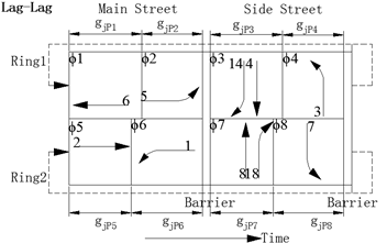
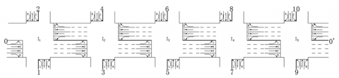
Since the lead left-turn PSP increases the delay of left-turning traffic on the artery, the lag-lag left-turn PSP is widely used for TSC at signalized intersections [12, 13]. In general, no green arrow indication is needed for right-turning traffic. But the right-turning traffic from the sides could have an immense impact on the through traffic on the artery. Thus, this paper incorporates right-turn phases for both northbound and southbound traffics to arterial TSC. Figure 2 presents a typical lag-lag left-turn PSP of dual-ring structure.
Figure 2. A typical lag-lag left-turn PSP under a dual-ring structure (Mckay, 1960)
Note: $\mathrm{g}_{\mathrm{jPk}}$ is the green interval of phase k at intersection j.
Phases 1, 2, 5, and 6, located between the first pair of barriers, serve the approaches on the artery. The critical paths through the artery is the larger one between the path associated with phases 1 and 2 in ring 1, and that associated with phases 5 and 6 in ring 2.
Phases 3, 4, 7, and 8 are located between the second pair of barriers. Phases 3 and 7 have two flow ratios: one for through traffic and the other for right-turning traffic. The larger between the two is the phase flow ratio. The critical paths through the side streets is the larger one between the path associated with phases 3 and 4 in ring 1, and that associated with phases 7 and 8 in ring 2 [13].
2.2 Inbound and outbound traffics
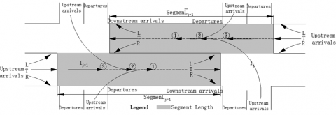
It is assumed that every traffic can merge into their destination lanes without having any conflict with another traffic. Take the outbound direction as an example. As shown in Figure 3, the inbound flows via the through lanes at intersection j come from three groups of traffics in the upstream interaction j-1 [14]: the through traffic on the artery, the left-turning traffic from the side, and the right-turning traffic from the side. Under any NEMA PSP, the through traffic from the upstream in the outbound direction is the last to arrive at the target intersection.
In the above PSP, the through lanes on the artery serve two kinds of traffic: the traffic from the sides, and the through traffic from the previous intersection in each direction. The latter arrives later than the first traffic. The green interval for the latter at the target intersection is proportional to the green interval for them at the previous intersection. The sequence of arriving traffics via the through lanes at the target intersection on the artery is explained below:
In outbound direction:
Intersection 1: 1. $\mathrm{q}_{1 \mathrm{th}}$.
Intersection j: 1. $\mathrm{q}_{\mathrm{j}-1 \mathrm{r}, \mathrm{jth}}$, 2. $\mathrm{q}_{\mathrm{j}-1 \mathrm{l}, \mathrm{jth}}$, …, 2j-3. $\mathrm{q}_{1 \mathrm{r}, \mathrm{jth}}$, 2j-2. $\mathrm{q}_{1l, \mathrm{th}}$, 2j-1. $\mathrm{q}_{1 \mathrm{th}, \mathrm{jth}}$.
In inbound direction:
Intersection i: 1. $\overline{\mathrm{q}}_{\mathrm{ith}}$.
Intersection j: 1. $\overline{\mathrm{q}}_{\mathrm{j}+1 \mathrm{r}, \mathrm{jth}}$, 2. $\overline{\mathrm{q}}_{\mathrm{j}+1l, \mathrm{jth}}$, …, 2(i-j)-1. $\overline{\mathrm{q}}_{\mathrm{ir}, \mathrm{jth}}$, 2(i-j). $\overline{\mathrm{q}}_{\mathrm{il}, \mathrm{jth}}$, 2(i-j)+1. $\overline{\mathrm{q}}_{\mathrm{ith}, \mathrm{jth}}$.
where, $\mathrm{q}_{1 \text { th }}$ is the traffic volume via the through lanes in the outbound direction at intersection 1 (veh/h); $\mathrm{q}_{\mathrm{kr}, \mathrm{jth}}$ is the traffic volume via the through lanes in outbound direction at intersection j and from the northbound direction of intersection k (veh/h); $\mathrm{q}_{\mathrm{kl}, \mathrm{jth}}$ is the traffic volume via the through lanes in outbound direction at intersection j and from the southbound direction of intersection k (veh/h); $\mathrm{q}_{\mathrm{kth}, \mathrm{jth}}$ is the traffic volume via the through lanes in outbound direction at intersection j and from the outbound direction of intersection k (veh/h); $\overline{\mathrm{q}}_{\mathrm{ith}}$ is the traffic volume via the through lanes in inbound direction at intersection i (veh/h); $\overline{\mathrm{q}}_{\mathrm{kr}, \mathrm{jth}}$ is the traffic volume via the through lanes in inbound direction at intersection j and from the southbound direction of intersection k (veh/h); $\overline{\mathrm{q}}_{\mathrm{kl}, \mathrm{jth}}$ is the traffic volume via the through lanes in inbound direction at intersection j and from the northbound direction of intersection k (veh/h); $\overline{\mathrm{q}}_{\mathrm{kth}, \mathrm{jth}}$ is the traffic volume via the through lanes in inbound direction at intersection j and from the inbound direction of intersection k (veh/h).
Figure 3. The traffic movements under lag-lag left-turn PSP on the artery
Note: Segment $L_{j}$ is the length of artery segment $L_{j}$ in the outbound direction; Segment $\bar{L}_{j}$ is the length of artery segment $\bar{L}_{j}$ in the inbound direction.
2.3 Start/end-time of green interval
According to the continuum flow model [15, 16], the green intervals of phases 1 and 5 were associated with the through traffic volume at intersection j on the artery, such that the outbound traffics on through lanes at intersection j could proceed through continuous intersections, when the signals at those intersections are green. The end-time of green interval of phases 1 and 5 at intersection j depends on the travel time in the last segment [17]:
$\mathrm{g}_{\mathrm{jp} 5} \geq \frac{\mathrm{q}_{\mathrm{jth}}}{\mathrm{s}_{\mathrm{th}}} \mathrm{C}, \mathrm{g}_{\mathrm{jp} 1} \geq \frac{\overline{\mathrm{q}}_{\mathrm{jth}}}{\overline{\mathrm{s}}_{\mathrm{th}}} \mathrm{C}$. (1)
$\mathrm{g}_{\mathrm{jP} 1}^{\mathrm{end}}=\mathrm{g}_{\mathrm{iP} 1}^{\mathrm{end}}+\sum_{\mathrm{k}=\mathrm{i}-1}^{\mathrm{j}} \overline{\mathrm{t}}_{\mathrm{segment} \mathrm{k}}$, $\mathrm{g}_{\mathrm{jP} 5}^{\mathrm{end}}=\mathrm{g}_{1 \mathrm{P} 5}^{\mathrm{end}}+\sum_{\mathrm{k}=1}^{\mathrm{j}-1} \mathrm{t}_{\mathrm{segment} \mathrm{k}}$. (2)
where, gipk is the green interval of phase $\mathrm{k} ; \mathrm{s}_{\mathrm{th}}$ and $\overline{\mathrm{s}}_{\mathrm{th}}$ are the saturated flow rates of through lane in outbound and inbound directions of the artery, respectively; $\mathrm{g}_{\mathrm{jPk}}^{\text {end }}$ is the end-time of green interval in phase $\mathrm{k}$ (a cyclic value); $\mathrm{t}_{\text {segment } \mathrm{k}}$ and $\overline{\mathrm{t}}_{\text {segment } \mathrm{k}}$ are the travel times of segment $\mathrm{k}$ in outbound and inbound directions of the artery, respectively; $\mathrm{C}$ is the common cycle length $C \geq \max \left(C_{j}, j=1,2, \ldots, i\right)\left(C_{j}\right.$ is the optimal cycle length of isolated intersection j obtained by Webster's model).
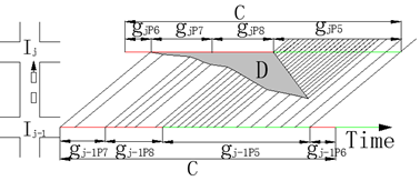
As shown in Figure $4,$ the start/end-time of green interval at the target intersection can be described by [18]:
$\left\{\begin{array}{l}\mathrm{g}_{\mathrm{jP} 5}^{\mathrm{end}}-\mathrm{g}_{\mathrm{jP} 5}=\mathrm{g}_{\mathrm{jP} 5}^{\mathrm{Start}} \\ \mathrm{g}_{\mathrm{jP} 1}^{\mathrm{end}}-\mathrm{g}_{\mathrm{jP} 1}=\mathrm{g}_{\mathrm{jP} 1}^{\mathrm{start}}\end{array}\right.$ (3)
$\mathrm{g}_{\mathrm{jP} 5}^{\mathrm{start}}=\mathrm{g}_{\mathrm{jP} 1}^{\text {start }}$ (4)
where, $\mathrm{g}_{\mathrm{jPk}}^{\mathrm{start}}$ is the start-time of green interval in phase k (a cyclic value).
Figure 4. The time-space diagram
Note: D is the total delay.
3.1 Optimal end-time of progressive green intervals for phase 1
According to the critical paths and flow ratios of intersection j, the minimum and maximum green intervals of phases 1 and 5 can be computed by [19]:
$\left\{\begin{array}{c}\mathrm{g}_{\mathrm{p} 1}^{\min }=\mathrm{y}_{\mathrm{j} 1} \times \mathrm{C} \\ \mathrm{g}_{\mathrm{jP} 1}^{\max }=\mathrm{C}-\left(\max \left(\mathrm{y}_{\mathrm{j} 3}+\mathrm{y}_{\mathrm{j} 4}, \mathrm{y}_{\mathrm{j} 7}+\mathrm{y}_{\mathrm{j} 8}\right)+\mathrm{y}_{\mathrm{j} 2}\right) \mathrm{C}, \mathrm{j}=1,2, \ldots \mathrm{i}\end{array}\right.$ (5)
$\left\{\begin{array}{c}\mathrm{g}_{\mathrm{jP}}^{\min }=\mathrm{y}_{\mathrm{j} 5} \times \mathrm{C} \\ \mathrm{g}_{\mathrm{jP}}^{\max }=\mathrm{C}-\left(\max \left(\mathrm{y}_{\mathrm{j} 3}+\mathrm{y}_{\mathrm{j} 4}, \mathrm{y}_{\mathrm{j} 7}+\mathrm{y}_{\mathrm{j} 8}\right)+\mathrm{y}_{\mathrm{j} 6}\right) \mathrm{C}, \mathrm{j}=1,2, \ldots, \mathrm{i}\end{array}\right.$ (6)
$\mathrm{g}_{\mathrm{jP} 1}^{\min } \leq \mathrm{g}_{\mathrm{jP} 1} \leq \mathrm{g}_{1 \mathrm{P} 1}^{\max }, \mathrm{g}_{\mathrm{j} \mathrm{P} 5}^{\min } \leq \mathrm{g}_{\mathrm{jP} 5} \leq \mathrm{g}_{1 \mathrm{P} 5}^{\max }$ (7)
where, $y_{j k}$ is the critical flow ratio for phase $k$ of intersection $j$ $\mathrm{g}_{\mathrm{jPk}}^{\min }$ and $\mathrm{g}_{\mathrm{jPk}}^{\max }$ are the minimum and maximum green intervals of phase k, respectively.
Figure 5. The end-time of green intervals for phases 1 and 5
Figure 6. The end band for phase 1
Under the constraints of the green intervals at the intersections, the maximum green intervals for phases 1 and 5 at intersections 1 and i were modified by [20]:
In outbound direction:
$\begin{aligned} \mathrm{W}_{\mathrm{j}} &=\frac{\sum_{\mathrm{k}=1}^{\mathrm{j}-1}\left(\mathrm{q}_{\mathrm{kr}, \mathrm{jth}}+\mathrm{q}_{\mathrm{kl}, \mathrm{jth}}\right)}{\mathrm{n} \times \mathrm{s}_{\mathrm{th}}} \\ & \mathrm{j}=2,3, \ldots, \mathrm{i}, \mathrm{W}_{1}=0 \end{aligned}$ (8)
$A_{j}=1-\max \left(y_{j, 3}+y_{j, 4}, y_{j, 7}+y_{j, 8}\right)-y_{j, 6}-W_{j}$ $j=1,2, \ldots, i$ (9)
$B_{j}=\frac{q_{1} t h, j t h}{n \times s_{t h}} j=1,2, \ldots, i$ (10)
$\mathrm{F}_{\mathrm{j}}=\frac{\mathrm{A}_{\mathrm{j}}}{\mathrm{B}_{\mathrm{j}}} \mathrm{j}=1,2, \ldots, \mathrm{i}$ (11)
$\mathrm{g}_{1 \mathrm{P} 5}^{\max ^{\prime}}=\mathrm{g}_{1 \mathrm{P} 5}^{\min } \times \min \left(\mathrm{F}_{1}, \mathrm{~F}_{2}, \ldots, \mathrm{F}_{\mathrm{i}}\right)$ (12)
$\mathrm{g}_{1 \mathrm{P} 5}^{\min } \leq \mathrm{g}_{1 \mathrm{P}_{5}} \leq \mathrm{g}_{1 \mathrm{P} 5}^{\max ^{\prime}}$ (13)
The green interval for phase 5 consists of three parts:
$\mathrm{t}_{\mathrm{j} 1}=\mathrm{B}_{\mathrm{j}} \times \mathrm{k} \times \mathrm{C} \quad 1 \leq \mathrm{k} \leq \min \left(\mathrm{F}_{1}, \mathrm{~F}_{2}, \ldots, \mathrm{F}_{\mathrm{i}}\right)$ (14)
$\mathrm{t}_{\mathrm{j} 2}=\mathrm{W}_{\mathrm{j}} \times \mathrm{C}$ (15)
$\mathrm{t}_{\mathrm{j} 3}=\mathrm{g}_{\mathrm{j} \mathrm{P} 5}^{\max }-\mathrm{t}_{\mathrm{j} 1}-\mathrm{t}_{\mathrm{j} 2}$ (16)
In outbound direction:
$\begin{aligned} \overline{\mathrm{W}}_{\mathrm{j}} &=\frac{\sum_{\mathrm{k}=\mathrm{i}}^{\mathrm{j}+1}\left(\overline{\mathrm{q}}_{\mathrm{kr}, \mathrm{th}}+\overline{\mathrm{q}}_{\mathrm{kl}, \mathrm{jth}}\right)}{\overline{\mathrm{n}} \times \overline{\mathrm{s}}_{\mathrm{th}}} \\ \mathrm{j} &=1,2, \ldots, \mathrm{i}-1, \mathrm{~W}_{\mathrm{i}}=0 \end{aligned}$ (17)
$\overline{\mathrm{A}}_{\mathrm{j}}=1-\max \left(\mathrm{y}_{\mathrm{j}, 3}+\mathrm{y}_{\mathrm{j}, 4}, \mathrm{y}_{\mathrm{j}, 7}+\mathrm{y}_{\mathrm{j}, 8}\right)-\mathrm{y}_{\mathrm{j}, 2}-\overline{\mathrm{W}}_{\mathrm{j}}$ $\mathrm{j}=1,2, \ldots, \mathrm{i}$ (18)
$\overline{\mathrm{B}}_{\mathrm{j}}=\frac{\overline{\mathrm{q}}_{\mathrm{ith}, \mathrm{jth}}}{\overline{\mathrm{n}} \times \overline{\mathrm{s}}_{\mathrm{th}}} \mathrm{j}=1,2, \ldots, \mathrm{i}$ (19)
$\overline{\mathrm{F}}_{\mathrm{j}}=\frac{\overline{\mathrm{A}}_{\mathrm{j}}}{\overline{\mathrm{B}}_{\mathrm{j}}} \mathrm{j}=1,2, \ldots, \mathrm{i}$ (20)
$\mathrm{g}_{\mathrm{iP} 1}^{\max ^{\prime}}=\mathrm{g}_{\mathrm{iP} 1}^{\min } \times \min \left(\overline{\mathrm{F}}_{1}, \overline{\mathrm{F}}_{2}, \ldots, \overline{\mathrm{F}}_{\mathrm{i}}\right)$ (21)
$\mathrm{g}_{\mathrm{iP} 1}^{\max ^{\prime}}=\mathrm{g}_{\mathrm{iP} 1}^{\min } \times \min \left(\overline{\mathrm{F}}_{1}, \overline{\mathrm{F}}_{2}, \ldots, \overline{\mathrm{F}}_{\mathrm{i}}\right)$ (22)
The green interval for phase 1 consists of three parts:
$\overline{\mathrm{t}}_{\mathrm{j} 1}=\overline{\mathrm{B}}_{\mathrm{j}} \times \overline{\mathrm{k}} \times \mathrm{C} \quad 1 \leq \overline{\mathrm{k}} \leq \min \left(\overline{\mathrm{F}}_{1}, \overline{\mathrm{F}}_{2}, \ldots, \overline{\mathrm{F}}_{\mathrm{i}}\right)$ (23)
$\overline{\mathrm{t}}_{\mathrm{j} 2}=\overline{\mathrm{W}}_{\mathrm{j}} \times \mathrm{C}$ (24)
$\overline{\mathrm{t}}_{\mathrm{j} 3}=\mathrm{g}_{\mathrm{jP} 1}^{\max }-\overline{\mathrm{t}}_{\mathrm{j} 1}-\overline{\mathrm{t}}_{\mathrm{j} 2}$ (25)
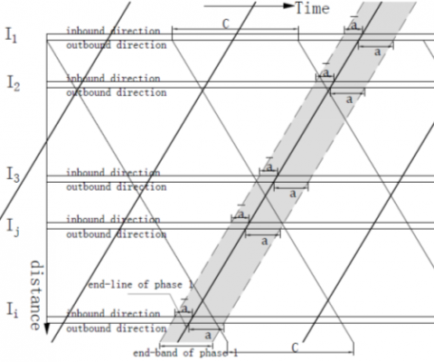
To facilitate the optimization of traffic progression band, the end-time of green intervals for phases 1 and 5 are presented in Figure 5. The set of alternating end-time of green intervals for phase 1 at intersections can be defined as [21]:
$\mathrm{g}_{\mathrm{jP} 1}^{\mathrm{eed}} \in\left[-\mathrm{g}_{\mathrm{jP} 5}^{\max }+\mathrm{g}_{\mathrm{jP} 1}^{\min },-\mathrm{g}_{\mathrm{jP}^{5}}^{\min }+\mathrm{g}_{\mathrm{jP} 1}^{\max }\right] \mathrm{j}=2,3, \ldots, \mathrm{i}-1$ (26)
$\mathrm{g}_{1 \mathrm{P} 1}^{\mathrm{end}} \in\left[-\mathrm{g}_{1 \mathrm{P} 5}^{\mathrm{max}^{\prime}}+\mathrm{g}_{\mathrm{jP} 1}^{\mathrm{min}},-\mathrm{g}_{\mathrm{jP} 5}^{\mathrm{min}}+\mathrm{g}_{\mathrm{jP} 1}^{\max }\right]$ (27)
$\mathrm{g}_{\mathrm{iP} 1}^{\mathrm{end}} \in\left[-\mathrm{g}_{\mathrm{iP} 5}^{\max }+\mathrm{g}_{\mathrm{jP} 1}^{\min },-\mathrm{g}_{\mathrm{jP} 5}^{\min }+\mathrm{g}_{\mathrm{jP} 1}^{\max ^{\prime}}\right]$ (28)
Under the constraint of $\mathrm{g}_{\mathrm{jP} 1}^{\mathrm{end}}=\mathrm{g}_{\mathrm{i} \mathrm{P} 1}^{\mathrm{end}}+\sum_{\mathrm{k}=\mathrm{i}-1}^{\mathrm{j}} \overline{\mathrm{t}}_{\mathrm{segment} \mathrm{k}}$, the end time of progressive green intervals (end band) for phase 1 was determined as shown in Figure 5. To balance the traffic in two directions, the end band weights for phase 1 were defined as $\theta_{\mathrm{P} 1}$ and $\bar{\theta}_{\mathrm{P} 1}$, which help to optimize the end band for phase 1:
$\theta_{\mathrm{P} 1}=\frac{\frac{\mathrm{q}_{1 \mathrm{th}}}{\mathrm{s}_{\mathrm{th}}}}{\frac{\mathrm{q}_{1 \mathrm{th}}}{\mathrm{s}_{\mathrm{th}}}+\frac{\overline{\mathrm{q}}_{\mathrm{i} \mathrm{th}}}{\overline{\mathrm{s}}_{\mathrm{th}}}}$ (29)
$\bar{\theta}_{\mathrm{P} 1}=\frac{\frac{\overline{\mathrm{q}}_{\mathrm{ith}}}{\overline{\mathrm{s}} \mathrm{th}}}{\frac{\mathrm{q}_{1 \mathrm{th}}}{\mathrm{s}_{\mathrm{th}}}+\frac{\overline{\mathrm{q}}_{\mathrm{ith}}}{\overline{\mathrm{s}}_{\mathrm{th}}}}$ (30)
Based on the end band weights, the end band was split into two parts a and $\overline{\mathbf{a}}$ (Figure 6):
$\mathrm{a}=\theta_{\mathrm{P} 1} \times \mathrm{t}_{\mathrm{P} 1}^{\mathrm{end}}$ (31)
$\overline{\mathrm{a}}=\bar{\theta}_{\mathrm{P} 1} \times \mathrm{t}_{\mathrm{P} 1}^{\mathrm{end}}$ (32)
where, $\mathrm{t}_{\mathrm{P} 1}^{\mathrm{end}}$ is the end band width of phase 1 (s).
3.2 Optimal start-time of progressive green intervals for phases 1 and 5
The green intervals for phases 1 and 5 can be computed by:
$\mathrm{g}_{\mathrm{jP} 1}^{\mathrm{start}}=\mathrm{g}_{\mathrm{j} \mathrm{P} 5}^{\mathrm{start}}=\max \left(\mathrm{g}_{\mathrm{jP} 5}^{\mathrm{end}}-\mathrm{g}_{\mathrm{j} \mathrm{P} 5}^{\mathrm{max}}, \mathrm{g}_{\mathrm{jP} 1}^{\mathrm{end}}-\mathrm{g}_{\mathrm{jP} 1}^{\max }\right)$
$\mathrm{j}=2,3, \ldots, \mathrm{i}-1$ (33)
$\mathrm{g}_{1 \mathrm{P} 1}^{\mathrm{start}}=\mathrm{g}_{1 \mathrm{P} 5}^{\mathrm{start}}=\max \left(\mathrm{g}_{1 \mathrm{P} 5}^{\mathrm{end}}-\mathrm{g}_{1 \mathrm{P} 5}^{\max ^{\prime}}, \mathrm{g}_{1 \mathrm{P} 1}^{\mathrm{end}}-\mathrm{g}_{1 \mathrm{P} 1}^{\max }\right)$ (34)
$\mathrm{g}_{\mathrm{iP} 1}^{\mathrm{start}}=\mathrm{g}_{\mathrm{iP} 5}^{\mathrm{start}}=\max \left(\mathrm{g}_{\mathrm{iP} 5}^{\mathrm{end}}-\mathrm{g}_{\mathrm{jP} 5}^{\mathrm{max}}, \mathrm{g}_{\mathrm{iP} 1}^{\mathrm{end}}-\mathrm{g}_{\mathrm{iP} 1}^{\max ^{\prime}}\right)$ (35)
$\mathrm{g}_{\mathrm{jP}_{5}}=\mathrm{g}_{\mathrm{jP} 5}^{\mathrm{end}}-\mathrm{g}_{\mathrm{jP} 5}^{\mathrm{start}}$ (36)
$\mathrm{g}_{\mathrm{jP} 1}=\mathrm{g}_{\mathrm{jP} 1}^{\mathrm{end}}-\mathrm{g}_{\mathrm{jP} 1}^{\mathrm{start}} \mathrm{j}=1,2, \ldots, \mathrm{i}$ (37)
Under the constraints of the above green intervals, $\mathrm{g}_{1 \mathrm{P} 5}$ and $\mathrm{g}_{\mathrm{iP} 1}$ were adjusted by:
$\mathrm{O}_{\mathrm{j}}=\frac{\mathrm{g}_{\mathrm{j} \mathrm{P}}-\mathrm{W}_{\mathrm{j}} \times \mathrm{C}}{\mathrm{B}_{\mathrm{j}} \times \mathrm{C}} \mathrm{j}=1,2, \ldots, \mathrm{i}, \mathrm{W}_{1}=0$ (38)
$\mathrm{g}_{1 \mathrm{P} 5}^{\prime}=\mathrm{g}_{1 \mathrm{P} 5}^{\min } \times \min \left(\mathrm{O}_{\mathrm{j}}, \mathrm{j}=1,2, \ldots, \mathrm{i}\right)$ (39)
$\mathrm{g}_{1 \mathrm{P} 1}^{\mathrm{start}}=\mathrm{g}_{1 \mathrm{P} 5}^{\mathrm{start}}=\mathrm{g}_{1 \mathrm{P} 5}^{\mathrm{end}}-\mathrm{g}_{1 \mathrm{P} 5}^{\prime}$ (40)
$\overline{\mathrm{O}}_{\mathrm{j}}=\frac{\mathrm{g}_{\mathrm{P} 1}-\overline{\mathrm{W}}_{\mathrm{j}} \times \mathrm{C}}{\overline{\mathrm{B}}_{\mathrm{j}} \times \mathrm{C}} \mathrm{j}=1,2, \ldots, \mathrm{i}$ (41)
$\mathrm{g}_{\mathrm{iP} 1}^{\prime}=\mathrm{g}_{\mathrm{iP} 1}^{\min } \times \min \left(\overline{\mathrm{O}}_{\mathrm{j}}, \mathrm{j}=1,2, \ldots, \mathrm{i}\right)$ (42)
$\mathrm{g}_{\mathrm{iP} 1}^{\mathrm{start}}=\mathrm{g}_{\mathrm{iP} 5}^{\mathrm{start}}=\mathrm{g}_{1 \mathrm{P} 1}^{\mathrm{end}}-\mathrm{g}_{1 \mathrm{P} 1}^{\prime}$ (43)
The green intervals for phase 5 at intersection 1 and those for phase 1 at intersection i should be recalculated, if they cause changes to minimal $\mathrm{O}_{\mathrm{j}}$ and $\overline{\mathrm{O}}_{\mathrm{j}}$.
To verify its applicability, the proposed efficient OD band model was tested on a typical artery network (Figure 7), using the estimated OD matrix in Table 1 [22, 23]. The lengths of the segments are as follows: $\mathrm{L}_{\text {segment } 1}=\overline{\mathrm{L}}_{\text {segment } 1}=300 \mathrm{~m}$, $\mathrm{L}_{\text {segment } 2}=\overline{\mathrm{L}}_{\text {segment } 2}=600 \mathrm{~m}, \mathrm{~L}_{\text {segment } 3}=\overline{\mathrm{L}}_{\text {segment } 3}=300 \mathrm{~m}$, and $\mathrm{L}_{\text {segment } 4}=\overline{\mathrm{L}}_{\text {segment } 4}=600 \mathrm{~m}$. The mean traffic speed was set to $60 \mathrm{~km} / \mathrm{h} .$ Thus, the travel time on each segment was obtained as: $t_{\text {segment1 }}=\overline{\mathrm{t}}_{\text {segment1 }}=18 \mathrm{~s}, \quad \mathrm{t}_{\text {segment } 2}=$$\overline{\mathrm{t}}_{\text {segment } 2}=32 \mathrm{~s}, \mathrm{t}_{\text {segment } 3}=\overline{\mathrm{t}}_{\text {segment } 3}=18 \mathrm{~s},$ and $\mathrm{t}_{\text {segment } 4}=$$\overline{\mathrm{t}}_{\text {segment } 4}=32 \mathrm{~s}$.
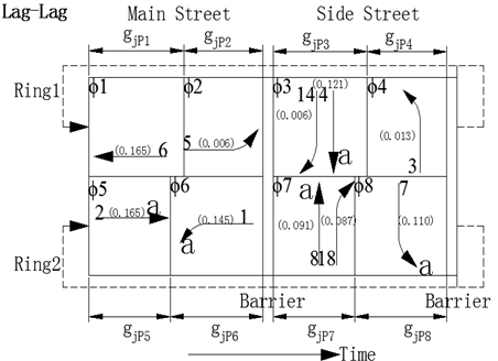
Moreover, the lag-lag PSP was adopted in the case study. Assuming that $\mathrm{s}_{\mathrm{th}}=\overline{\mathrm{s}}_{\mathrm{th}}$=1,650veh/h/ln, the data in intersection 1 were selected as an example to calculate the critical traffic flow ratios and critical phases (Figure 8).
Assuming that C=80s, the maximum and minimum green intervals for phases 1 and 5 were calculated (Table 2).
Under the constraints of the above green intervals, the maximum green interval for phase 1 at intersection i and that for phase 5 at intersection 1 were modified (Table 3).
Assuming that $\mathrm{g}_{1 \mathrm{P} 5}^{\text {end }}=0+\mathrm{nC}, \quad$ then $\mathrm{g}_{2 \mathrm{P} 5}^{\mathrm{end}}=18+\mathrm{nC}$, $\mathrm{g}_{3 \mathrm{P} 5}^{\mathrm{end}}=54+\mathrm{nC}, \mathrm{g}_{4 \mathrm{P} 5}^{\mathrm{end}}=72+\mathrm{nC}$ and, $\mathrm{g}_{5 \mathrm{P} 5}^{\mathrm{end}}=108+\mathrm{nC}$. The set of alternating end-time can be calculated as: $\mathrm{g}_{1 \mathrm{P} 1}^{\text {end }} \in$$[-29+\mathrm{nC}, 49+\mathrm{nC}], \mathrm{g}_{2 \mathrm{P} 1}^{\text {end }} \in[-8+\mathrm{nC}, 58+\mathrm{nC}], \mathrm{g}_{3 \mathrm{P} 1}^{\text {end }} \in$$[23,+\mathrm{nC}, 88+\mathrm{nC}], \mathrm{g}_{4 \mathrm{P} 1}^{\text {end }} \in[39+\mathrm{nC}, 101+\mathrm{nC}], \mathrm{g}_{5 \mathrm{P} 1}^{\text {end }} \in$$[75+\mathrm{nC}, 138+\mathrm{nC}]$.
since $\mathrm{g}_{\mathrm{jP} 1}^{\mathrm{end}}=\mathrm{g}_{\mathrm{iP} 1}^{\mathrm{end}}+\sum_{\mathrm{k}=\mathrm{i}-1}^{\mathrm{j}} \overline{\mathrm{t}}_{\mathrm{segment} \mathrm{k}},$ and intersections 1 and 4 are critical intersections, the green intervals of the end band for phase 1 at the intersections of the artery (Figure 9) can be obtained as: $\mathrm{g}_{1 \mathrm{P} 1}^{\mathrm{end}} \in[111+\mathrm{n} \mathrm{C}, 129+\mathrm{nC}], \mathrm{g}_{2 \mathrm{P} 1}^{\mathrm{end}} \in$$[93+\mathrm{nC}, 111+\mathrm{nC}], \mathrm{g}_{2 \mathrm{P} 1}^{\mathrm{end}} \in[57+\mathrm{nC}, 75+\mathrm{nC}], \mathrm{g}_{4 \mathrm{P} 1}^{\mathrm{end}} \in$$[39+\mathrm{nC}, 57+\mathrm{nC}], \mathrm{g}_{5 \mathrm{P} 1}^{\mathrm{end}} \in[3+\mathrm{nC}, 21+\mathrm{nC}]$.
For phase $1,$ the progressive end band lasts $18 \mathrm{~s}$. The values of $\theta_{\mathrm{P} 1}$ and $\bar{\theta}_{\mathrm{P} 1}$ were computed as: $\theta_{\mathrm{P} 1}=41.5 \%,$ and $\bar{\theta}_{\mathrm{P} 1}=$$58.5 \% .$ Then, it can be derived that $a=11,$ and $\bar{a}=7$ (Figure 10).
From the values of $\theta_{P 1}$ and $\bar{\theta}_{P 1},$ the end-time of the progressive green intervals can be obtained as: $\mathrm{g}_{1 \mathrm{P} 1}^{\text {end }}=202+$$\mathrm{nC}, \mathrm{g}_{2 \mathrm{P} 1}^{\mathrm{end}}=184+\mathrm{nC}, \mathrm{g}_{3 \mathrm{P} 1}^{\mathrm{end}}=148+\mathrm{nC}, \mathrm{g}_{4 \mathrm{P} 1}^{\mathrm{end}}=130+\mathrm{nC}$$\mathrm{g}_{5 \mathrm{P} 1}^{\mathrm{end}}=94+\mathrm{nC}$.
Since the green intervals of phases 1 and 5 start at the same moment, the start-time can be obtained by: $\mathrm{g}_{1 \mathrm{P} 1}^{\text {start }}=\mathrm{g}_{1 \mathrm{P} 5}^{\mathrm{start}}=$$139+\mathrm{nC}, \quad \mathrm{g}_{2 \mathrm{P} 1}^{\mathrm{start}}=\mathrm{g}_{2 \mathrm{P} 5}^{\mathrm{start}}=125+\mathrm{nC}, \quad \mathrm{g}_{3 \mathrm{P} 1}^{\mathrm{start}}=\mathrm{g}_{3 \mathrm{P} 5}^{\mathrm{start}}=$$90+\mathrm{nC}, \mathrm{g}_{4 \mathrm{P} 1}^{\mathrm{start}}=\mathrm{g}_{4 \mathrm{P} 5}^{\mathrm{start}}=93+\mathrm{nC}, \mathrm{g}_{5 \mathrm{P} 1}^{\mathrm{start}}=\mathrm{g}_{5 \mathrm{P} 5}^{\mathrm{stat}}=55+nC$.
So, $\mathrm{g}_{1 \mathrm{P} 1}^{1}=63, \overline{\mathrm{O}}_{1}=5.50, \mathrm{~g}_{1 \mathrm{P} 5}^{1}=21, \mathrm{O}_{1}=1.50 ; \mathrm{g}_{2 \mathrm{P} 1}^{1}=59$, $\overline{\mathrm{O}}_{2}=3.46, \mathrm{~g}_{2 \mathrm{P} 5}^{1}=53, \quad \mathrm{O}_{2}=3.54 ; \mathrm{g}_{3 \mathrm{P} 1}^{1}=58, \quad \overline{\mathrm{O}}_{3}=$$3.13, \mathrm{~g}_{3 \mathrm{P} 5}^{1}=44, \mathrm{O}_{2}=2.82 ; \mathrm{g}_{4 \mathrm{P} 1}^{1}=37, \overline{\mathrm{O}}_{4}=1.65, \mathrm{~g}_{4 \mathrm{P} 5}^{1}=59$, $\mathrm{O}_{4}=5.11 ; \mathrm{g}_{5 \mathrm{P} 1}^{1}=39, \overline{\mathrm{O}}_{5}=1.95, \mathrm{~g}_{5 \mathrm{P} 5}^{1}=53, \mathrm{O}_{5}=5.63$.
The value of $\mathrm{O}_{1}$ is the minimum among $\mathrm{O}_{\mathrm{j}},$ while the value of $\bar{O}_{4}$ is the minimum among $\bar{O}_{j}$. Hence, the green intervals of phase 5 at intersection 1 and phase 1 at intersection 5 can be respectively calculated by: $\mathrm{g}_{1 \mathrm{P} 5}^{\prime}=\mathrm{g}_{1 \mathrm{P} 5}^{\min } \times \mathrm{O}_{1}=21, \mathrm{~g}_{5 \mathrm{P} 1}^{\prime}=$$g_{\mathrm{iP} 1}^{\min } \times \overline{\mathrm{O}}_{4}=32$.
Since the green intervals of the two phases start at the same moment, the green interval was changed to 46s. The change for phase 5 at intersection 1 did not affect the value of $\mathrm{O}_{1}$; the change for phase 1 at intersection 5 caused the value of $\mathrm{O}_{1}$ to change to 4.75, but did not affect the minimum of $\overline{0}_{j}$. The final results are displayed in Table 4.
Figure 11 presents the progressive green intervals, under which all the traffics on the through lanes can proceed through all intersections without meeting any red light.
Figure 7. The typical arterial network
Figure 8. The determination of critical paths
Note: a is the critical traffic flow ratio.
Figure 9. The green intervals of the end band for phase 1 at the intersections of the artery
Figure 10. The Results of a and $\overline{\mathbf{a}}$
Figure 11. The progressive green intervals
Table 1. The estimated OD matrix of the arterial network (veh/h)
|
OD |
0 |
1 |
2 |
3 |
4 |
5 |
6 |
7 |
8 |
9 |
10 |
0’ |
|
0 |
0 |
50 |
10 |
5 |
15 |
60 |
15 |
50 |
10 |
10 |
30 |
350 |
|
1 |
20 |
0 |
150 |
10 |
10 |
15 |
20 |
0 |
10 |
10 |
20 |
40 |
|
2 |
10 |
200 |
0 |
5 |
0 |
10 |
0 |
10 |
20 |
60 |
15 |
50 |
|
3 |
20 |
10 |
0 |
0 |
200 |
5 |
0 |
20 |
15 |
30 |
30 |
70 |
|
4 |
50 |
40 |
10 |
200 |
0 |
10 |
30 |
20 |
40 |
20 |
10 |
30 |
|
5 |
50 |
30 |
30 |
40 |
5 |
0 |
250 |
10 |
50 |
30 |
40 |
30 |
|
6 |
70 |
20 |
35 |
20 |
0 |
200 |
0 |
0 |
10 |
5 |
10 |
10 |
|
7 |
50 |
5 |
30 |
10 |
20 |
5 |
10 |
0 |
180 |
35 |
20 |
60 |
|
8 |
10 |
10 |
50 |
0 |
5 |
20 |
10 |
210 |
0 |
20 |
15 |
20 |
|
9 |
50 |
0 |
10 |
40 |
30 |
35 |
20 |
40 |
60 |
0 |
200 |
60 |
|
10 |
25 |
30 |
50 |
15 |
10 |
20 |
15 |
5 |
10 |
150 |
0 |
50 |
|
0’ |
400 |
80 |
40 |
50 |
30 |
60 |
50 |
20 |
70 |
50 |
60 |
0 |
Table 2. The time intervals of $g_{j \mathrm{P} 1}^{\min } / \mathrm{g}_{\mathrm{j} \mathrm{P} 1}^{\max }$ and $\mathrm{g}_{\mathrm{j} \mathrm{P} 5}^{\min } / \mathrm{g}_{\mathrm{jP} 5}^{\max }(\mathrm{s})$
|
|
Time intervals |
||||
|
I1 |
I2 |
I3 |
I4 |
I5 |
|
|
$\mathrm{g}_{\mathrm{jP} 1}^{\min } / \mathrm{g}_{\mathrm{jP} 1}^{\max }(\mathrm{s})$ |
18/63 |
27/ 60 |
26/58 |
26/55 |
20/46 |
|
$\mathrm{g}_{\mathrm{jP} 5}^{\min } / \mathrm{g}_{\mathrm{jP} 5}^{\max }(\mathrm{s})$ |
14/52 |
20/53 |
24/55 |
22/59 |
16/53 |
Table 3. The variables values and maximum green intervals for phases 1 and 5
|
Intersection |
Direction |
Variable values and maximal green intervals for phases 1 and 5 |
|||||
|
$\mathrm{W}_{\mathrm{j}} / \overline{\mathrm{W}}_{\mathrm{j}}$ |
$\mathrm{A}_{\mathrm{j}} / \overline{\mathrm{A}}_{\mathrm{j}}$ |
$\mathrm{B}_{\mathrm{j}} / \overline{\mathrm{B}}_{\mathrm{j}}$ |
$\mathrm{F}_{\mathrm{j}} / \overline{\mathrm{F}}_{\mathrm{j}}$ |
$\mathrm{t}_{\mathrm{j} 2} / \overline{\mathrm{t}}_{\mathrm{j} 2}(\mathrm{~s})$ |
$\mathrm{g}_{\mathrm{iP} 1}^{\max ^{\prime}} / \mathrm{g}_{1 \mathrm{P} 5}^{\max ^{\prime}}(\mathrm{s})$ |
||
|
I1 |
Inbound |
0.10 |
0.69 |
0.12 |
5.79 |
8 |
|
|
Outbound |
0.00 |
0.65 |
0.17 |
3.96 |
0 |
47 |
|
|
I2 |
Inbound |
0.17 |
0.59 |
0.16 |
3.70 |
14 |
|
|
Outbound |
0.08 |
0.58 |
0.16 |
3.63 |
7 |
|
|
|
I3 |
Inbound |
0.14 |
0.60 |
0.18 |
3.34 |
11 |
|
|
Outbound |
0.16 |
0.53 |
0.14 |
3.89 |
13 |
|
|
|
I4 |
Inbound |
0.11 |
0.58 |
0.22 |
2.71 |
9 |
|
|
Outbound |
0.15 |
0.59 |
0.12 |
5.01 |
13 |
|
|
|
I5 |
Inbound |
0.00 |
0.58 |
0.24 |
2.38 |
0 |
46 |
|
Outbound |
0.09 |
0.57 |
0.11 |
5.41 |
8 |
|
|
Table 4. The final results of $\mathrm{g}_{\mathrm{jP} 1}^{\mathrm{start}}, \mathrm{g}_{\mathrm{jP} 1}^{\mathrm{end}}, \mathrm{g}_{\mathrm{jP} 5}^{\mathrm{start}}, \mathrm{g}_{\mathrm{jP} 5}^{\mathrm{end}}, \mathrm{g}_{\mathrm{jP} 1},$ and $\mathrm{g}_{\mathrm{jP} 5}$
|
Intersection |
$\mathrm{g}_{\mathrm{jP} 1} / \mathrm{g}_{\mathrm{jP}_{5}}(\mathrm{~s})$ |
$\mathrm{g}_{\mathrm{jP} 1}^{\mathrm{start}} / \mathrm{g}_{\mathrm{jP}^{5}}^{\mathrm{start}}$ |
$\mathrm{g}_{\mathrm{jP} 1}^{\mathrm{end}} / \mathrm{g}_{\mathrm{jP} 5}^{\mathrm{end}}$ |
|
I1 |
63 |
59+nC |
122+nC |
|
21 |
59+nC |
80+nC |
|
|
I2 |
59 |
45+nC |
104+nC |
|
53 |
45+nC |
98+nC |
|
|
I3 |
58 |
90+nC |
148+nC |
|
44 |
90+nC |
134+nC |
|
|
I4 |
37 |
93+nC |
130+nC |
|
59 |
93+nC |
152+nC |
|
|
I5 |
32 |
142+nC |
174+nC |
|
46 |
142+nC |
188+nC |
The efficient OD band model has the following advantages over the previous methods:
(1) Based on the estimated OD matrix, the dynamics of through traffic and turning-in/out traffic on the artery are analyzed under the lag-lag PSP, producing the traffic movement sequence at continuous intersections. Since the through traffic from the previous intersection arrives later at the target intersection of the artery than the turning-in traffic, two kinds of traffic are considered to determine the green interval for traffics on through lanes at intersections: the traffic from the sides, and the through traffic from the previous intersection in each direction. The green interval for the latter at the target intersection is proportional to the green interval for them at the previous intersection.
(2) The end-time of the green intervals at continuous intersections form a straight line, such that all through traffics can pass through these intersections without meeting any red light. According to the relationship between the start/end-time of green interval and the minimum/maximum green intervals, the set of alternating end-time of green intervals for phase 1 at intersections is obtained, and then decomposed by the weight of traffic demand in each direction of the artery.
(3) The maximum green interval for through traffic at the target intersection on the artery is constrained by that at any other intersection, due to the proportionality between the green intervals for the said two kinds of traffics. In addition, the green intervals of phases 1 and 5 start at the same moment. In this way, the progression band produced by our model enables the through and turning-in/out traffics to proceed through continuous intersections, when the signals at those intersections are green.
To sum up, the efficient OD band model provides a novel tool to obtain bi-directional progression bands for traffic with heavy turning movements on the artery. The obtained bands are asymmetric and of variable bandwidth. The case study demonstrates that the proposed model can effectively satisfy the demand of actual traffic flow through simple calculations, and output intuitive progression bands. The future research will consider the lost time of arterial traffics and the walking time of pedestrians in the design of progression band, and study the progression band under patterns other than NEMA PSP.
This work was funded by the Philosophy and Social Sciences Foundation of Tianjin, China (Grant No.: TJGL16-014Q).
[1] Little, J.D. (1966). The synchronization of traffic signals by mixed-integer linear programming. Operations Research, 14(4): 568-594. https://doi.org/10.1287/opre.14.4.568
[2] Morgan, J.T., Little, J.D. (1964). Synchronizing traffic signals for maximal bandwidth. Operations Research, 12(6): 896-912. https://doi.org/10.1287/opre.12.6.896
[3] Gartner, N.H., Assman, S.F., Lasaga, F., Hou, D.L. (1991). A multiband approach to arterial traffic signal optimization. Transportation Research Part B: Methodological, 25(1): 55-74. https://doi.org/10.1016/0191-2615(91)90013-9
[4] Little, J.D., Kelson, M.D., Gartner, N.H. (1981). MAXBAND: A versatile program for setting signals on arteries and triangular networks. Transportation Research Record: Journal of the Transportation Research Board, 795: 40-46. http://hdl.handle.net/1721.1/1979
[5] Arsava, T., Xie, Y., Gartner, N.H. (2016). Arterial progression optimization using OD-BAND: Case study and extensions. Transportation Research Record, 2558(1): 1-10. https://doi.org/10.3141/2558-01
[6] Lu, K., Zheng, S.J., Xu, J.M., Li, L. (2011). Green wave coordinated control optimization models oriented to different bi-directional bandwidth demands. Journal of Traffic and Transportation Engineering, 11(5): 101-108. https://doi.org/10.1080/0144929X.2011.553739
[7] Chen, N.N., He, Z.C., Yu, Z. (2009). Revised MAXBAND model considered variable queue clearance time. Journal of Wuhan University of Technology (Transportation Science and Engineering), 33(5): 843-847. https://doi.org/10.3963/j.issn.1006-2823.2009.05.008
[8] Zhang, C., Xie, Y., Gartner, N.H., Stamatiadis, C., Arsava, T. (2015). AM-band: an asymmetrical multiband model for arterial traffic signal coordination. Transportation Research Part C: Emerging Technologies, 58: 515-531. https://doi.org/10.1016/j.trc.2015.04.014.
[9] Arsava, T., Xie, Y., Gartner, N.H., Mwakalonge, J. (2014). Arterial traffic signal coordination utilizing vehicular traffic origin-destination information. In 17th International IEEE Conference on Intelligent Transportation Systems (ITSC), pp. 2132-2137. https://doi.org/10.1109/itsc.2014.6958018
[10] Hu, P., Tian, Z., Yuan, Z., Jia, S. (2011). Variable-bandwidth progression optimization in traffic operation. Jounal of Transportation Systems Engineering and Information Technology, 11(1): 61-72. https://doi.org/10.1016/S1570-6672(10)60101-8
[11] Ding, N., He, Q., Wu, C. (2014). Performance measures of manual multimodal traffic signal control. Transportation Research Record, 2438(1): 55-63. https://doi.org/10.3141/2438-06
[12] Mckay, B.W. (1968). Lead and lag left turn signals. Traffic Safety Research Review, 38(7): 50, 52-53, 56. https://trid.trb.org/view/113565
[13] Washington, D. (2000). Highway capacity manual. Special Report, 1(1-2): 5-7. http://dx.doi.org/10.9774/GLEAF.978-1-909493-38-4_2
[14] Liu, Y., Chang, G.L. (2011). An arterial signal optimization model for intersections experiencing queue spillback and lane blockage. Transportation Research Part C: Emerging Technologies, 19(1): 130-144. https://doi.org/10.1016/j.trc.2010.04.005
[15] Qu, D.Y., Wan, M.F., Wang, Z.L., Xu, X.H., Wang, J.Z. (2017). Green wave coordinate control method for arterial traffic based on traffic wave theory. Journal of Highway and Transportation Research and Development, 11(4): 65-73. https://doi.org/10.3969/j.issn.1002-0268.2016.09.018
[16] Kachroo, P., Özbay, K. (1999). Traffic flow theory. Advances in Industrial Control, Springer, London, 19-43. https://doi.org/10.1007/978-1-4471-0815-3_2
[17] Sun, M., Yang, F., Bei, D., Ge, T. (2013). Analysis of queue dissipation time effect based on traffic wave theory. Journal of Highway and Transportation Research and Development, 30(10): 112-116. https://doi.org/10.3969/j.issn.1002-0268.2013.10.020
[18] Zhang, Y., Li, S. (1999). Analysis of congestion and dissipation at signalized intersections. Journal of Changsha Communications University, 15(3): 57-61. https://doi.org/10.3969/j.issn.1674-599X.1999.03.013
[19] Wu, B., Li, Y. (2009). Traffic Management and Control. China Communications Press, Beijing.
[20] Liu, X., Tang, S. (2012). Green wave coordinated control method based on continuously passing vehicles. Journal of Transportation Systems Engineering and Information Technology, 12(6): 34-40. https://doi.org/10.16097/j.cnki.1009-6744.2012.06.019
[21] Cao, J.J., Han, Y., Yao, J. (2015). A dynamic dual-direction green wave optimization control model for urban arterial roads. Journal of Highway and Transportation Research and Development, 32(9): 115-120. https://doi.org/10.3969/j.issn.1002-0268.2015.09.019
[22] Chen, D.Y., Chen, G.R., Wang, Y.W. (2013). Real-time dynamic vehicle detection on resource-limited mobile platform. IET Computer vision, 7(2): 81-89. https://doi.org/10.1049/iet-cvi.2012.0088
[23] Wang, Y., Tian, Z. (2020). Optimization method of coordinated control for signalized intersection based on NEMA phase. Chinese patent: CN201710768162.3,2020-9-20.