Assem Thabet* | Ghazi Bel Haj Frej | Noussaiba Gasmi | Brahim Metoui
© 2020 IIETA. This article is published by IIETA and is licensed under the CC BY 4.0 license (http://creativecommons.org/licenses/by/4.0/).
OPEN ACCESS
This brief discusses a simple stabilization strategy for a class of Lipschitz nonlinear systems based on the transformation of nonlinear function to Linear Parameter Varying system. Due to the introduction of the Differential Mean Value Theorem (DMVT), the dynamic and output nonlinear functions are transformed into Linear Parameter Varying (LPV) functions. This allows to increase the number of decision variables in the constraint to be resolved and, then, get less conservative and more general Linear Matrix Inequality (LMI) conditions. The established sufficient stability conditions are in the form of LMI with the introduction of a cost control to ensure closed-loop stability. Finally, Real Time Implementation (RTI) using a DSP device (ARDUINO UNO R3) to a typical robot is given to illustrate the performances of the proposed method with a comparison to some existing results.
Lipchitz nonlinear systems, cost control, stabilization, nonlinear-observer, real-time-implementation
The principle of supervision of nonlinear systems (control, state estimation, diagnosis ...) have been exploited in many monitoring areas and industrial control which they are based mostly on feedback principle using state or/and output-feedback controllers [1-5].
In recent years, the feedback stabilization, tracking and control problem [6-10] has attracted the attention of many researchers due to the importance of its applications. This area of research remains a field which knows a development and an important success. Special attention is devoted to Lipschitz nonlinear systems.
Effectively, for nonlinear systems that verify the Lipchitz properties, different methods and solid approaches have been treated as: adaptive design [11-15], extended-state-observer with back-stepping [16, 17], finite-time control [18], neural network control [19, 20], H∞ fuzzy-logic [21], non-fragile passive controller [22] and Petri Nets [23].
In spite of the important literature of the developed methods, several limitations still exist:
In this brief, a strategy of observer-based control method for Lipschitz nonlinear systems with a guarantee cost control is proposed. The considered systems satisfy the Lipschitz property. This paper is based partially on the works of these papers [6, 24]. The main contribution lies in the use of DMVT on nonlinear functions terms which transformed to Linear Parameter Varying (LPV) functions. This allows introducing additional decision variables to enhance the constraint to be resolved. The convergence of the augmented error to zero is ensured by the use Lyapunov theory and the convexity principle (LMI) while optimizing a quadratic criterion taking into account the interconnection between the state and the control. This method can be extended to more general class of nonlinear systems verifying the Lipschitz properties (singular, distributed, decentralized).
This brief is organized as follows: In the next part of this section, some useful preliminaries are presented. The second section introduces the problem formulation and the synthesis methodology of the proposed approach is detailed. This approach is based on the LMIs feasibility conditions. Finally, Real Time Implementation (RTI) using a DSP device (ARDUINO UNO R3) to a typical robot is given to illustrate the performances of the proposed method with a comparison to some existing results.
Notations:
We consider the following notations in this brief:
$e_{s}(j)=$$\left(\begin{array}{c}j^{t h} \\ \underbrace{0, \ldots, 0,1,0, \ldots, 0} \\ s-c o m p o n e n t s\end{array}\right)^{T}$$\in \mathbb{R}^{s}$ , s≥1, is the vector of the canonical basis of $\mathbb{R}^{s}$.
The set of equations of a general class of nonlinear system is given by:
$\left\{\begin{array}{l}\dot{x}=g(t, x)+B u \\ y=h(x, u)\end{array}\right.$ (1)
where, $x \in \mathbb{R}^{n}$ the state vector, $u \in \mathbb{R}^{m}$: input and $y(t) \in \mathbb{R}^{p}$ output. The matrix B is constant with adequate dimension.
$g(t, x): \mathbb{R}^{n} \times \mathbb{R}^{n} \rightarrow \mathbb{R}^{n}$ and $h(x, u): \mathbb{R}^{n} \times \mathbb{R}^{m} \rightarrow \mathbb{R}^{p}$ are nonlinear vectors fields (supposed differentiable to x).
Considering the following assumptions and proposals:
Assumption 1: The Jacobian matrices of g(.) and h(.) satisfy [25]:
$\left\{\begin{array}{l}-\infty<\underline{g}_{i j} \leq \frac{\partial g_{i}(t, x)}{\partial x_{j}} \leq \bar{g}_{i j}<+\infty \\ -\infty<\underline{h}_{i j} \leq \frac{\partial h_{i}(x, u)}{\partial x_{j}} \leq \bar{h}_{i j}<+\infty\end{array}\right.$ (2)
where,
$\underline{g}_{i j}=\min _{F \in \mathbb{R}^{n} \times \mathbb{R}^{n}}\left(\frac{\partial g_{i}}{\partial x_{j}}(F)\right) ; \bar{g}_{i j}=\max _{F \in \mathbb{R}^{n} \times \mathbb{R}^{n}}\left(\frac{\partial g_{i}}{\partial x_{j}}(F)\right)$
$\underline{h}_{i j}=\min _{F \in \mathbb{R}^{n} \times \mathbb{R}^{m}}\left(\frac{\partial h_{i}}{\partial x_{j}}(F)\right) ; \bar{h}_{i j}=\max _{F \in \mathbb{R}^{n} \times \mathbb{R}^{m}}\left(\frac{\partial h_{i}}{\partial x_{j}}(F)\right)$
Proposition 1. [24]: Let $f: \mathbb{R}^{n} \rightarrow \mathbb{R}^{k}$ and $x_{1}, x_{2} \in \mathbb{R}^{n}$. If f is differentiable in $\operatorname{Co}\left(x_{1}, x_{2}\right)$, then, there are constant vectors $r_{1}, \ldots, r_{k} \in \operatorname{Co}\left(x_{1}, x_{2}\right)$, $r_{i} \neq x_{1}$, $r_{i} \neq x_{2}$ for $i=1, \ldots, k$ with:
$f\left(x_{1}\right)-f\left(x_{2}\right)=\left(\sum_{i, j=1}^{k, n} e_{k}(i) e_{n}^{T}(j) \frac{\partial f_{i}}{\partial x_{j}}\left(r_{i}\right)\right)\left(x_{1}-x_{2}\right)$ (3)
Proposition 2. [24]: Let the two sets $D_{n, n}$ and $E_{p, n}$ be defined as follows:
$\left\{\begin{aligned} D_{n, n}=&\left\{a=\left(a_{11}, \ldots, a_{1 n}, \ldots, a_{n n}\right)\right.\\ &\left.: \underline{g}_{i j} \leq a_{i j} \leq \bar{g}_{i j}, i=1, \ldots, n ; j=1, \ldots, n ;\right\} \\ E_{p, n}=&\left\{b=\left(b_{11}, \ldots, b_{1 n}, \ldots, b_{p n}\right)\right.\\ &\left.\vdots \underline{h}_{i j} \leq b_{i j} \leq \bar{h}_{i j}, i=1, \ldots, p ; j=1, \ldots, n ;\right\} \end{aligned}\right.$ (4a)
The sets of vertices of $D_{n, n}$ and $E_{p, n}$ (supposed a bounded convex domain) are given by:
$\left\{\begin{aligned} \mathcal{W}_{E_{p, n}}=\left\{c=\left(c_{11}, \ldots, c_{1 n}, \ldots, c_{p n}\right):\right.\\\left.c_{i j} \in\left\{\underline{h}_{i j}, \bar{h}_{i j}\right\}\right\} \\ \mathcal{V}_{D_{n, n}}=\{d=\left(d_{11}, \ldots, d_{1 n}, \ldots, d_{n n}\right): \\ \left.d_{i j} \in\left\{\underline{g}_{i j}, \bar{g}_{i j}\right\}\right\} \end{aligned}\right.$ (4b)
This gives
$\mathcal{A}_{L}(a)=\sum_{i, j=1}^{n, n} a_{i j} e_{n}(i) e_{n}^{T}(j)$
$\mathcal{G}(b)=\sum_{i, j=1}^{p, n} b_{i j} e_{p}(i) e_{n}^{T}(j)$ (5)
where, $\mathcal{A}_{L}(a)$ and $\mathcal{G}(b)$ are the affine matrices functions.
In the next section, the proposed approach will be detailed to synthesis of observer / control gains that guarantee closed-loop stability.
3.1 Method design
The proposed observer for system (1) is described by:
$\left\{\begin{array}{l}\dot{\hat{x}}=B u+L(y-\hat{y})+g(t, \hat{x}) \\ \hat{y}=h(\hat{x}, u)\end{array}\right.$ (6)
where, $\hat{x}$ and L are the estimated state and the observation gain matrix respectively.
Now, let’s define $\varepsilon=x-\hat{x}$ as the variation of dynamic state estimation error. Using (6) and (1), we obtain:
$\dot{\varepsilon}=\Delta g-L \Delta h$ (7)
and $\Delta g=g(t, x)-g(t, \hat{x})$ and $\Delta h=h(x, u)-h(\hat{x}, u)$. Now, using Proposition 1 on g(.) and h(.) and knowing that there exists $\left(r_{i}(t), \bar{r}_{i}(t)\right) \in C o(x, \hat{x})$, for all $i=1 \ldots n$, we obtain:
$\left\{\begin{array}{l}\Delta h=h(x, u)-h(\hat{x}, u)=\left(\sum_{i, j=1}^{p, n} e_{p}(i) e_{n}^{T}(j) \frac{\partial h}{\partial x_{j}}\left(\bar{r}_{i}\right)\right) \varepsilon \\ \Delta g=g(t, x)-g(t, \hat{x})=\left(\sum_{i, j=1}^{n, n} e_{n}(i) e_{n}^{T}(j) \frac{\partial g}{\partial x_{j}}\left(r_{i}\right)\right) \varepsilon\end{array}\right.$ (8)
Note: Let’s consider the notation:
$z_{i j}(t)=\frac{\partial h_{i}}{\partial x_{j}}\left(\bar{r}_{i}(t), u\right) ; z(t)=\left(z_{11}(t), \ldots, z_{1 n}(t), . . z_{p n}(t)\right)$
$w_{i j}(t)=\frac{\partial g_{i}}{\partial x_{j}}\left(r_{i}(t)\right) ; w(t)=\left(w_{11}(t), . ., w_{1 n}(t), . . w_{n n}(t)\right)$
Then, using (5) and (8) in (7), gives:
$\dot{\varepsilon}=\left(\mathcal{A}_{L}(w(t))-L \mathcal{G}(z(t))\right) \varepsilon$ (9)
Which leads to that the observer design of systems (1) is transformed into stability problem of LPV systems (9) which offered by the use of DMVT.
In the next step we are interested in the development of control gain matrix. To do so, the following expression is a typical form of state feedback control:
$u=-K \hat{x}$ (10)
with $K \in \mathbb{R}^{m \times n}$ is the control gain matrix. Including this control form (10) in the nonlinear system, we can obtain:
$\left\{\begin{array}{l}\dot{x}=-B K x+B K \varepsilon+g(t, x) \\ y=h(x, u)\end{array}\right.$ (11)
Similarly, using Proposition 1, the function $g(t, x)$ is equivalent to $g(t, x)-g\left(t_{0}, 0\right)$ assuming that $g\left(t_{0}, 0\right)=0$ where:
$g(t, x)-g\left(t_{0}, 0\right)=\left(\sum_{i, j=1}^{n, n} e_{n}(i) e_{n}^{T}(j) \frac{\partial g}{\partial x_{j}}\left(r_{i}\right)\right) x$
where, $r_{i} \in C o(x, 0)$ which allows to have: $g(t, x)=\mathcal{A}_{C}(w(t)) x$. Therefore, including the overall system (11) and the dynamics observation error system (9), the augmented system is given by:
$\underbrace{\left[\begin{array}{c}\dot{x} \\ \dot{\varepsilon}\end{array}\right]}_\tilde{x}=\underbrace{\left[\begin{array}{cc}\mathcal{A}_{C}(w(t))-B K & B K \\ 0 & \mathcal{A}_{L}(w(t))-L \mathcal{G}(z(t))\end{array}\right]}_\tilde{A} \underbrace{\cdot\left[\begin{array}{l}x \\ \varepsilon\end{array}\right]}_\tilde{x}$ (12)
The next section presents the synthesis method of different parameters through a transformation to a convex optimization algorithm (LMIs) with two steps.
3.2 Stability analysis
This part is devoted to the stability analysis while ensuring optimization of a cost control. The criterion to optimize is as follows:
$J=\int_{0}^{\infty}\left(\left[\begin{array}{ll}x & u\end{array}\right]^{T}\left(\begin{array}{ll}Q & S \\ S^{T} & R\end{array}\right)\left[\begin{array}{ll}x & u\end{array}\right] d t\right.$ (13)
With $Q=Q^{T}>0$, $S>0$ and $R=R^{T}>0$ are constant weighting matrices.
Note: In contrary to standard methods, this cost control considers that the state and the control are interconnected.
Now, using the form $u=-K \hat{x}$, the cost control (13) is developed as follows:
$\tilde{J}=\int_{0}^{\infty}\left(\tilde{x}^{T}\underbrace{\left[\begin{array}{cc}Q+K^{T} R K-S K-(S K)^{T} & -K^{T} R K+S K \\ -K^{T} R K+(S K)^{T} & K^{T} R K\end{array}\right]}_\tilde{Q} \tilde{x} \mid d t\right.$ (14)
Based on Yang et al. [26], the state feedback control is explored to be a quadratic guaranteed cost control with a positive cost for the augmented system (12) using (13) if the closed loop system is stable. This is guaranteed if and only if $J<\tilde{J}$ for all admissible nonlinearities.
First, we define the candidate Lyapunov function $V(\tilde{x})$:
$V(\tilde{x})=\tilde{x}^{T} P \tilde{x}$ (15)
With P is given by:
$P=\left[\begin{array}{cc}P_{c} & 0 \\ 0 & P_{0}\end{array}\right]$
where, $P_{c}=P_{c}^{T}$ and $P_{0}=P_{0}^{T}$ are Lyapunov SDP matrices. The aim is to satisfy this inequality:
$\frac{d}{d t} V(\tilde{x})+\tilde{x}^{T} \tilde{Q} \tilde{x}<0$ (16)
From (15) and (16), we obtain:
$(\tilde{A} \tilde{x})^{T} P \tilde{x}+\tilde{x}^{T} P(\tilde{A} \tilde{x})+\tilde{x}^{T} \tilde{Q} \tilde{x}<0$ (17)
Then, the condition for the asymptotic stability [26] with a guaranteed level of performance is given by:
$\tilde{x}^{T}\left(\tilde{A}^{T} P+P \tilde{A}+\tilde{Q}\right) \tilde{x}<0$ (18)
The main result is given by the following theorem:
Theorem 1:
The system (1) is stable by guaranteeing the cost control (13) in the sense of Lyapunov if there are matrices of appropriate dimensions P=PT, L and K where the following LMI has solution:
$b l k-\operatorname{diag}\left(G\left(d^{1}, c^{1}\right), \ldots, G\left(d^{2^{q n}}, c^{2^{p n}}\right)\right)<0,$
$d^{i} \in \mathcal{V}_{D_{q, n}}$ for $i=1, \ldots, 2^{q n}$
$c^{j} \in \mathcal{W}_{E_{p, n}}$ for $j=1, \ldots, 2^{p n}$
$G\left(d^{i}, c^{j}\right)=\tilde{A}\left(d^{i}, c^{j}\right)^{T} P+P \tilde{A}\left(d^{i}, c^{j}\right)+\tilde{Q}$ (19)
Proof:
Eq. (19) can be rewritten in the form of the following block matrix:
$\left(\begin{array}{ll}Z_{11} & Z_{12} \\ Z_{21} & Z_{22}\end{array}\right)<0$ (20)
With:
$\left\{\begin{aligned} Z_{11}=& \mathcal{A}_{C}(d)^{T} P_{c}+P_{c} \mathcal{A}_{C}(d)-K^{T} B^{T} P_{c}-P_{c} B K+Q \\ &+K^{T} R K-(S K)^{T}+K S \\ Z_{12}=& P_{c} B K-K^{T} R K+K S \\ Z_{21}=& X_{12}^{T} \\ Z_{22}=& \mathcal{A}_{L}(d)^{T} P_{0}+P_{0} \mathcal{A}_{L}(d)-\mathcal{G}(c)^{T} L^{T} P_{0}-P_{0} L \mathcal{G}(c) \\ &+K^{T} R K \end{aligned}\right.$
Now, let’s proceed to a resolution algorithm with two steps:
- Introducing a new S-variable and pre- and post-multiplying (20) by:
$\left(\begin{array}{cc}M & 0 \\ 0 & I\end{array}\right), M=M^{T}=P_{c}^{-1}>0$ (21)
This leads to:
$\left(\begin{array}{ll}T_{11} & T_{12} \\ T_{21} & T_{22}\end{array}\right)<0$ (22)
Considering the change of variables: N=KM and V=P0L, the result will be:
$\left\{\begin{aligned} T_{11}=& M \mathcal{A}_{C}(d)^{T}+\mathcal{A}_{C}(d) M-N^{T} B^{T}-B N \\ &+M Q M+N^{T} R N+N^{T} S^{T} M W+M S N \\ T_{12}=& B K-N^{T} R K+M S K \\ T_{21}=& T_{12}^{T} \\ T_{22}=& \mathcal{A}_{L}(d)^{T} P_{0}+P_{0} \mathcal{A}_{L}(d)-\mathcal{G}(c)^{T} V^{T}-V \mathcal{G}(c) \\ &+K^{T} R K \end{aligned}\right.$
Now, the resolution of the matrix inequality T11<0 allows direct deduction of the matrices M and N.
Secondly, the application of the Schur complements [27], leads to:
The resolution of (23) gives the control gain matrix by K=NM-1.
$\left[\begin{array}{ccccccc}M \mathcal{A}_{C}(d)^{T}+\mathcal{A}_{C}(d) M -N^{T} B^{T}-B N & M & N^{T} & N^{T} & M \\ \star & -Q^{-1} & 0 & 0 & 0 \\ \star & 0 & -R^{-1} & 0 & 0 \\ \star & 0 & 0 & -\left(S^{T}\right)^{+} & 0 \\ \star & 0 & 0 & 0 & -S^{+}\end{array}\right]<0$ (23)
The next step of resolution and determination of the observer parameters (determination of P0 and V by the LMI (22)) is done by injecting the values of M and N (determined with the resolution of T11 <0). Thereafter, we will easily the observation gain L=P0-1V.
In order to validate the approach presented in this brief, an example will be considered with a real-time implementation by the use of DSP board ARDUINO UNO-R3 device as a real-time emulator (Hardware in the Loop) on a typical one-link flexible joint robot [28].
The dynamic equation for the system is given as:
$\left\{\begin{array}{l}\dot{x}(t)=A x(t)+B u(t)+g(x(t)) \\ y(t)=h(x(t), u(t))\end{array}\right.$
where, all the parameters and their physical meanings are given by the paper [27].
$A=\left[\begin{array}{cccc}-10 & 1 & 0 & 0 \\ -48.6 & -1.26 & 48.6 & 0 \\ 0 & 0 & -22 & 1 \\ 1.95 & 0 & -19.5 & -6\end{array}\right] ; B=\left[\begin{array}{l}0 \\ 1 \\ 0 \\ 0.5\end{array}\right]$
$h(x, u)=\left[\begin{array}{l}x_{1} \\ \sin \left(2 x_{2}\right)\end{array}\right] ; g(x(t))=\left[\begin{array}{l}0 \\ 0 \\ 0 \\ \gamma_{f} \sin \left(x_{3}\right)\end{array}\right]$
Now, Applying the DMVT approach with Lipschitz constant $\gamma_{f}=3.33$ leads to:
- $A x+g(t, x)=\mathcal{A}_{C}(w(t)) x$
- $D_{1 j}=0$ for all $j=1,2,3$; $D_{14}=\gamma_{f} \cos \left(r_{3}\right)$.
- $\mathcal{V}_{D_{1,4}}$ can be reduced to $\mathcal{V}_{D_{1,4}}=\left\{-\gamma_{f},+\gamma_{f}\right\}$ .
- For function $h(x, u)$: $\underline{h}_{2,2}=-2$ and $\bar{h}_{2,2}=2$ .
- The initial conditions are: $\mathrm{x}(0)=\left[\begin{array}{llll}0.5 & 0.5 & 0.5 & 0.5\end{array}\right]^{\mathrm{T}}$ ; $\hat{\mathrm{x}}(0)=[-0.5-0.5-0.5-0.5]^{\mathrm{T}}$ .
Now, the resolution of LMI (19) in Theorem 1, give:
$K=\left[\begin{array}{lll}-40.0473 & -17.8391 & -6.6076 & 42.08\end{array}\right]$ ;
$L=\left[\begin{array}{cc}0.0495 & -1.8578 \\ 0.0385 & 21.3563 \\ -0.0259 & -3.0453 \\ -0.0505 & -3.0309\end{array}\right]$
where, $Q=0.001 I_{4}$, $R=0.01$ and $\mathrm{S}=\left[\begin{array}{llll}0.1 & 0.1 & 0.1 & 0.1\end{array}\right]^{\mathrm{T}}$ .
For the real time implementation using the DSP device "ARDUINO UNO R3 device", all technical details and configuration steps with MATLAB / Simulink are given in the papers [6-9].
Note: In all the figures, the real state will be symbolized by a solid line and that estimated by dashed line and all magnitudes are in Volts.
The first step in this RTI consists in injecting a variable sinusoidal noise on the output of the system in terms of amplitude $\pm 10 \%$ of y and frequency 140Hz.
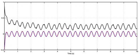
Figure 1 presents the variation of real x1 and its estimate ( $\hat{x}_{1}$ ).
Figure 1 present clearly that the state is very well estimated (despite very small variations which are due to disturbances). This result is deduced from the use of the DMVT on the nonlinear function allowing a scanning of the entire range of variation (operation) from two limit points (from $-\gamma_{f}$ to $\gamma_{f}$ ).
The second step in this RTI consists in interposing two additive sinusoidal noises variable in terms of frequency 240Hz and amplitude $\pm 30 \%$ . These two noises will be injected respectively on the dynamics of the system and the output. Figure 2 presents the evolution real x4 and its estimate ( $\hat{x}_{4}$ ) by the proposed design (dashed red line) and the method of [10] (dashed black line).
From Figure 2 can directly deduce that the proposed approach ensures the stabilization of the overall system even with the presence of variable noise during the first transient mode when the method [10] presents a biased result.
The third step in this RTI is to further amplify the two sinusoidal noises in terms of frequency (550Hz-3800Hz) and amplitude ±45%. These two noises will be injected as well as the second phase.
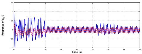
Figure 3 presents the real $x_{2}$ and its estimate ( $\hat{x}_{2}$ ).
From Figure 3 we deduce in a clear way that the system remains stable and converges the point of origin even by further amplifying the extreme disturbances that can be simulated in several real industrial cases.
Figure 1. Evolution of x1 and its estimate
Figure 2. Evolution of x4 and its estimate
Figure 3. Evolution of x2 and its estimate
The results provided in this section show clearly that the proposed approach ensures stabilization and convergence towards the equilibrium state even in the presence of disturbances of great value. This is guaranteed by the application of DMVT on the nonlinear dynamic and output functions. Indeed, this principle makes it possible to take into consideration the system transformed into LPV while scanning the different operating points in the interval of variation formed from two extreme limits of the Lipschitz constants.
In this paper, a simple stabilization approach for nonlinear systems which verify the Lipschitz condition is presented.
The transformation from a nonlinear system to an easily treatable LPV class is ensured through the use of DMVT. This allowed having nonrestrictive sufficient conditions on nonlinear functions during the synthesis of LMIs guaranteeing convergence towards the point of origin. This while ensuring the optimization of a quadratic criterion implementing a direct correlation between the state vector and that of input/control.
RTI with ARDUNO board which was used as an emulator confirms the high quality of stabilization offered by the proposed approach.
A further question needs to be investigated:
- The generalization of the proposed One-sided Lipschitz systems.
- An extension to adaptive control in Reciprocal Space systems framework (considering nonlinear outputs expressed with derivatives of states).
These extensions will be investigated (as part of a project) in the near future
[1] Wang, D., Pang, K., Wang, W., Zhang, Y., Yao, W., Zhao, L. (2020). Development and application of an internal fault detection system for transformer based on wall climbing robot. European Journal of Electrical Engineering, 22(2): 193-198. https://doi.org/10.18280/ejee.220213
[2] Mahapatra, S., Subudhi, B. (2017). Design and experimental realization of a backstepping nonlinear H∞ control for an autonomous underwater vehicle using a nonlinear matrix inequality approach. Transactions of the Institute of Measurement and Control, 40(1): 3390-3403. https://doi.org/10.1177/0142331217721315
[3] Schmidt, P., Moreno, J., Schaum, A. (2014). Observer design for a class of complex networks with unknown topoloy. World Congress the International Federation of Automatic Control, Cape Town, South Africa, pp. 2812-2817. https://doi.org/10.3182/20140824-6-ZA-1003.01716
[4] Gripa, H.F., Saberi, A., Johansenb, T.A. (2012). Observers for interconnected nonlinear and linear systems. Automatica, 48(7): 1339-1346. https://doi.org/10.1016/j.automatica.2012.04.008
[5] Iovine, A., Siad, S., Damm, G., Santis, E., Benedetto, M. (2017). Nonlinear control of a DC microgrid for the integration of photovoltaic panels. IEEE Trans. Automation Science and Engineering, 149(2): 524-535. https://doi.org/10.1109/TASE.2017.2662742
[6] Thabet, A., Frej, G.B.H., Boutayeb, M. (2018). Observer-based feedback stabilization for Lipschitz nonlinear systems with extension to h∞ performance analysis: Design and experimental results. IEEE Trans. Control Systems Technology, 26(1): 321-328. https://doi.org/10.1109/TCST.2017.2669143
[7] Gasmi, N., Boutayeb, M., Thabet, A., Aoun, M. (2018). Enhanced LMI conditions for observer-based H∞ stabilization of Lipschitz discrete-time systems. European Journal of Control, 44: 80-89. https://doi.org/10.1016/j.ejcon.2018.09.016
[8] Gasmi, N., Thabet, A., Boutayeb, M., Aoun, M. (2015). Observer design for a class of nonlinear discrete time systems. IEEE Int. Conf. on Sciences and Techniques of Automatic Control and Computer Engineering, Monastir, Tunisia, pp. 799-804. https://doi.org/10.1109/STA.2015.7505084
[9] Gasmi, N., Boutayeb, M., Thabet, A., Aoun, M. (2019). Sliding window based nonlinear H∞ filtering: Design and experimental results. IEEE Transactions on Circuits and Systems II: Express Briefs, 66(2): 302-306. https://doi.org/10.1109/TCSII.2018.2859484
[10] Pagilla, P., Zhu, Y. (2004). Controller and observer design for Lipschitz nonlinear systems. Proceedings of the 2004 American Control Conference, Boston, Massachusetts, USA, pp. 2379-2384. https://doi.org/10.23919/ACC.2004.1383820
[11] Yao, B., Tomizuka, M. (2001). Adaptive robust control of MIMO nonlinear systems in semi-strict feedback forms. Automatica, 37(9): 1305-1321. https://doi.org/10.1016/S0005-1098(01)00082-6
[12] Li, D., Liu, Y., Tong, S., Chen, C., Li, D.J. (2018). Neural networks-based adaptive control for nonlinear state constrained systems with input delay. IEEE Trans. on Cybernetics, 49(4): 1249-1258. https://doi.org/10.1109/TCYB.2018.2799683
[13] Sakthivel, R., Selvaraj, P., Lim, Y., Karimi, H. (2017). Adaptive reliable output tracking of networked control systems against actuator faults. Journal of the Franklin Institute, 354(9): 3813-3837. https://doi.org/10.1016/j.jfranklin.2016.06.022
[14] Liu, Y., Lu, S., Tong, S., Chen, X., Chen, C., Li, D. (2018). Adaptive control-based barrier Lyapunov functions for a class of stochastic nonlinear systems with full state constraints. Automatica, 87: 83-93. https://doi.org/10.1016/j.automatica.2017.07.028
[15] Liu, Y., Tong, S. (2017). Barrier Lyapunov functions for Nussbaum gain adaptive control of full state constrained nonlinear systems. Automatica, 76: 143-152. https://doi.org/10.1016/j.automatica.2016.10.011
[16] Yao, J., Jiao, Z., Ma, D. (2014). Extended state observer-based output feedback nonlinear robust control of hydraulic systems with backstepping. IEEE Trans. on Industrial Electronics, 61(11): 6285-6293. https://doi.org/10.1109/TIE.2014.2304912
[17] Li, Y.F., Zheng, T.X., Li, Y.G. (2015). Extended state observer based adaptive back-stepping sliding mode control of electronic throttle in transportation cyber-physical systems. Mathematical Problems in Eng., 2015: 1-11. https://doi.org/10.1155/2015/301656
[18] Liu, H., Zhang, T., Tian, X. (2015). Continuous output-feedback finite time control for a class of second-order nonlinear systems with disturbances. International Journal of Robust and Nonlinear Control, 26(2): 185-364. https://doi.org/10.1002/mc.3305
[19] Ge, S., Hang, C., Zhang, T. (1999). Adaptive neural network control of nonlinear systems by state and output feedback. IEEE Trans. on Syst. Man and Cybernetics, 29(6): 818-828. https://doi.org/10.1109/3477.809035
[20] Li, D.P., Li, D.J. (2017). Adaptive neural tracking control for an uncertain state constrained robotic manipulator with unknown time-varying delays. IEEE Transactions on Systems, Man, and Cybernetics, 48(12): 2219-2228. https://doi.org/10.1109/TSMC.2017.2703921
[21] Kaewpraek, N., Assawinchaichote, W. (2016). H∞ fuzzy state-feedback control plus state-derivative-feedback control synthesis for photovoltaic systems. Asian Journal of Control, 18(4): 1441-1452. https://doi.org/10.1002/asjc.1233
[22] He, S.P. (2015). Non fragile passive controller design for nonlinear Markovian jumping systems via observer-based control. Neurocomputing, 147: 350-357. https://doi.org/10.1016/j.neucom.2014.06.053
[23] Giua, A., Seatzu, C., Basile, F. (2004). Observer-based state-feedback control of timed petri nets with deadlock recovery. IEEE Transactions on Automatic Control, 49(1): 17-29. https://doi.org/10.1109/TAC.2003.821419
[24] Zemouch, A., Boutayeb, M. (2009). A unified H∞ adaptive observer synthesis method for a class of systems with both Lipchitz and monotone nonlinearities. Syst. Control Letters, 58(4): 282-288. https://doi.org/10.1016/j.sysconle.2008.11.007
[25] Zemouch, A., Boutayeb, M., Bara, G. (2008). Observers for a class of Lipchitz systems with extension to H∞ performance analysis. Syst. Control Letters, 57(1): 18-27. https://doi.org/10.1016/j.sysconle.2007.06.012
[26] Yang, G.H., Wang, J.L., Soh, Y.C. (2000). Reliable guaranteed cost control for uncertain nonlinear systems. IEEE Transactions on Automatic Control, 45(11): 2188-3192. https://doi.org/10.1109/9.887682
[27] Boyd, S., Ghaoui, L.E., Ferron, E., Balakrishnan, V. (1994). Linear matrix Inequalities in Systems and Control Theory. 15th ed. Philadelphia: Studies in Applied Mathematics SIAM.
[28] Spong, M.W. (1987). Modeling and control of elastic joint robots. Trans. ASME, J. Dyn. Syst., Meas. Control, 109(4): 310-319. https://doi.org/10.1115/1.3143860