Fengmei Gao* | Pan Wu
© 2020 IIETA. This article is published by IIETA and is licensed under the CC BY 4.0 license (http://creativecommons.org/licenses/by/4.0/).
OPEN ACCESS
With the development of smart healthcare, surgical and rehabilitation robots have permeated into daily medical operations. This raises concerns over the trajectory planning of medical manipulators. Based on particle swarm optimization (PSO) algorithm and fuzzy neural network (FNN), this paper puts forward a trajectory planning algorithm for medical manipulators, which ensures that the target medical manipulator can suppress the residual jitter at the end, while meeting the requirements of high precision, flexible operation, and disturbance resistance. Specifically, a kinetic model was constructed for a medical manipulator of multi-degrees-of-freedoms (DOFs) through position and posture transforms, and used to construct an FNN for trajectory planning. To suppress the jitter at the end, an adaptive PSO algorithm was designed, and combined with the FNN into a trajectory planning algorithm called PSO neural network (PSONN) algorithm. Finally, the proposed algorithm was proved effective through experiments. The research results provide the reference for applying PSO algorithm and FNN in other fields.
particle swarm optimization (PSO) algorithm, medical manipulator, jitter suppression, fuzzy neural network (FNN)
With the rapid progress of artificial intelligence (AI) and computer technology, industrial robots have been gradually applied in various industries. The technology of industrial robots is increasing mature, as evidenced by the integration of multiple joints, central processing units (CPUs), and sensors [1-6].
Recently, medical robots and other medical equipment have attracted much attention. To assist doctors in surgeries, medical manipulators must be highly accurate and flexible, and good at jitter suppression [7-9], ensuring the stability and continuity of velocity and acceleration. Before the surgery, the manipulator trajectory must be optimized to minimize the impact on each joint, and to precisely reach the designated positions [10-12].
Currently, the trajectories of applied manipulators are mainly planned through obstacle avoidance by artificial potential field (APF) method, trajectory length calculation by ant colony algorithm, and accurate graph search based on machine vision [13-15]. Mohamed et al. [16] found the optimal solution to joint variables with distributed AI, and solved the reverse motion of a seven-degrees-of-freedom (DOFs) manipulator. Through nonuniform B-spline interpolation, Annisa et al. [17] optimized manipulator trajectory under the constraints of acceleration and torque, and thereby improved the real-time control effect of the manipulator. Using adaptive impedance, Annisa et al. [18] offset the effect of initial parameter values on manipulator control system, and increased the accuracy and velocity of repetitive manipulator motions through iterative learning. Jamali et al. [19] set up an object space coordinate system for a flexible robot platform, constructed a neural network (NN)-based impedance control strategy for different unknown disturbances, and expanded the applicable scope of the robot by adjusting the impedance.
To meet the needs and effects of surgeries, medical manipulators generally have multiple DOFs. The large number of DOFs poses a key difficulty in motion control and trajectory planning of medical manipulators. Therefore, many experts and scholars have attempted to balance the DOF, accuracy, flexibility, and jitter suppression of medical manipulators [20-23]. Based on the topology of constrained space, Wilkening et al. [24] modelled the DOFs of a flexible medical manipulator, and designed the structure of a variable rigidity medical manipulator, capable of multi-DOF motions and effective lock-up. Based on the real-time video images captured by the Vision Development Module of LabVIEW, Sefati et al. [25] carried out three-dimensional (3D) observation of the manipulator from multiple angles, and realized the real-time observation and control of the medical process.
Based on particle swarm optimization (PSO) algorithm and fuzzy neural network (FNN), this paper proposes a trajectory planning algorithm for medical manipulators called PSO neural network (PSONN) algorithm. The PSONN enables the target medical manipulator to adapt to the changes in system disturbances and suppress the residual jitter at the end, while meeting the requirements of high precision and flexible operation. Firstly, a kinetic model was built for a n-DOF medical manipulator through position and posture transforms, and used to construct an FNN for trajectory planning. To suppress the jitter at the end, an adaptive PSO algorithm was designed, and combined with the FNN to plan the trajectories of the medical manipulator. The proposed method was proved effective through experiments.
The DOFs of a manipulator refer to the number of independent motion parameters that must be given to describe the manipulator’s motion, turning or rotation. This number is often the same as that of driving mechanisms (hydraulic or electric motors). Each DOF corresponds to ae mechanical joint.
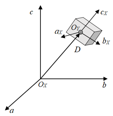
The workspace range of the manipulator depends on two factors: the length of each link and the configuration space of each joint. Hence, a reference CS X and the CS of the rigid link Y were set up for the manipulator workspace. Let vector D=[abc]T be any point in the workspace (See Figure 1).
Figure 1. The reference CS and rigid link CS
Then, the direction of the rigid link relative to CS X can be expressed as:
$P_{X-Y}=\left[\begin{array}{lll}X_{a_{Y}} & X_{b_{Y}} & X_{c_{Y}}\end{array}\right]=\left[\begin{array}{lll}u_{a} & v_{a} & w_{a} \\ u_{b} & v_{b} & w_{b} \\ u_{c} & v_{c} & w_{c}\end{array}\right]$ (1)
where, PX-Y is the transform matrix from CS Y to CS X. The matrix consists of the direction cosines of the three unit principal vectors XaY, XbY, and XcY relative to the CS X.
The position vector [abc] can be combined with formula (1) to illustrate the position and posture of the rigid link mapped from CS Y to CS X:
$H_{X-Y}=\left[\begin{array}{cc}P_{X-Y} & D \\ 0 & 1\end{array}\right]=\left[\begin{array}{cccc}u_{a} & v_{a} & w_{a} & a \\ u_{b} & v_{b} & w_{b} & b \\ u_{c} & v_{c} & w_{c} & c \\ 0 & 0 & 0 & 1\end{array}\right]$ (2)
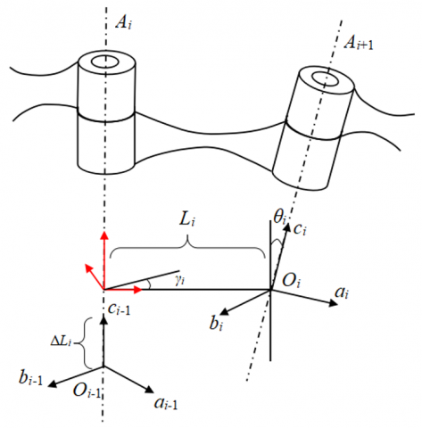
The medical manipulator is a multi-joint multi-DOF device with both flexible and rigid links. The transform matrix Wi between the two kinds of links can be described as:
$W_{i}=R\left(b, \gamma_{i}\right) * T\left(0,0, \Delta L_{i}\right) * T\left(L_{i}, 0,0\right) * R\left(a, \theta_{i}\right)$ (3)
where, Li is the length of the common perpendicular between the axis of the i-th joint Ai and that of the i+1-th joint Ai+1; θi is the angle between the axis of the i+1-th joint Ai+1 and the plane F made of the axis of the i-th joint Ai and the common perpendicular Li; ΔLi is the distance between the two common perpendiculars Li and Li-1 of the i-th joint Ai; γi is the angle between the projections of common perpendiculars Li and Li-1 on the plane with the axis of the axis of the i-th joint Ai as the normal.
Figure 2. The position and posture transforms of the link
As shown in Figure 2, the positions and angles of the link between the two joints can be transformed by Wi through two rotations (by θi about x-axis and γi about z-axis) and two translations (by Li and γi).
The cosine form of Wi can be expressed as:
$W_{i}=\left[\begin{array}{cccc}\cos \gamma_{i} & -\sin \gamma_{i} \cos \theta_{i} & \sin \gamma_{i} \sin \theta_{i} & L_{i} \cos \gamma_{i} \\ \sin \gamma_{i} & \cos \gamma_{i} \cos \theta_{i} & -\cos \gamma_{i} \sin \theta_{i} & L_{i} \sin \gamma_{i} \\ 0 & \sin \theta_{i} & \cos \theta_{i} & \Delta L_{i} \\ 0 & 0 & 0 & 1\end{array}\right]$ (4)
If the rigid connection position of CS Y is moved from the original end to the other end, formulas (3) and (4) can be transformed into:
$W_{i}=T\left(L_{i}, 0,0\right) * R\left(a, \theta_{i}\right) * T\left(0,0, \Delta L_{i}\right) * R\left(b, \gamma_{i}\right)$
$=\left[\begin{array}{cccc}\cos \theta_{\mathrm{i}} & -\sin \theta_{\mathrm{i}} & 0 & L_{\mathrm{i}-1} \\ \sin \gamma_{\mathrm{i}} \cos \theta_{i-1} & \cos \gamma_{i} \cos \theta_{i-1} & -\sin \theta_{i-1} & -\Delta L_{i} \sin \theta_{i-1} \\ \sin \gamma_{i} \sin \theta_{i-1} & \cos \gamma_{i} \sin \theta_{i-1} & \cos \theta_{i-1} & -\Delta L_{i} \cos \theta_{i-1} \\ 0 & 0 & 0 & 1\end{array}\right]$ (5)
To determine the joint parameters, position, and speed of the multi-link n-DOF medical manipulator, the end position and posture of each link can be solved by the transform matrix Wi of each link:
$W=W_{1} \cdot W_{2} \ldots W_{n}$ (6)
Substituting the total kinetic energy and total potential energy of the manipulator into the Lagrangian equation, the kinetic model of the manipulator can be established as:
$\sum_{i=1}^{n} J_{i}(\theta) \ddot{\theta}_{i}+C_{i}(\theta, \dot{\theta})+G_{i}(\theta)=\tau$ (7)
where, Ji, Ci, and Gi are the rotational inertia matrix, centripetal matrix, and gravity matrix of the i-th joint of the robotic arm, respectively; τi is the driving torque vector of the i-th joint of the i-th joint:
$J_{i}(\theta)=\left[\begin{array}{c}\left(m_{i}+m_{i+1}\right) L_{i+1}^{2}+m_{i+1} L_{i+1}^{2}+2 m_{i+1} L_{i} L_{i+1} \cos \theta_{i+1} \\ m_{i+1} L_{i+1}^{2}+m_{i+1} L_{i} L_{i+1} \cos \theta_{i+1} \\ m_{i+1} L_{i+1}^{2}+m_{i+1} L_{i 1} L_{i+1} \cos \theta_{i+1} \\ m_{i+1} L_{i+1}^{2}\end{array}\right.$ (8)
$C_{i}(\theta, \dot{\theta})=\left[\begin{array}{c}-m_{i+1} L_{i} L_{i+1}\left(2 \dot{\theta}_{i} \dot{\theta}_{i+1}+\dot{\theta}_{i+1}\right) \sin \theta_{i+1} \\ m_{i+1} L_{i} L_{i+1} \dot{\theta}_{i} \sin \theta_{i+1}\end{array}\right]$ (9)
$G_{i}(\theta)=\left[\begin{array}{c}m_{i} g L_{i} \cos \theta_{i}+m_{i+1} g L_{i+1} \cos \theta_{i+1} \\ m_{i+1} g L_{i+1} \theta_{i} \cos \theta_{i+1}\end{array}\right]$ (10)
where, mi, and mi+1 are the mass of the two links connected to the i-th joint, respectively; g is the acceleration of gravity.
To improve the trajectory control accuracy of the medical manipulator, this paper sets up an FNN based on the above kinetic model. As shown in Figure 3, the FNN consists of five layers, namely, an input layer, a fuzzification layer, a fuzzy inference layer, a normalization layer, and an output layer.
Figure 3. The structure of the FNN
The position and posture signals of each joint Oi(1)=xi, i=1, 2, …, N were imported to the input layer.
With M fuzzy control rules, the fuzzification layer performs fuzzification of the signals with a Gaussian membership function:
$\begin{aligned} O_{i j}^{(2)} &=\exp \left[-\frac{\left(x_{i}-a_{i j}\right)^{2}}{\sigma_{i j}^{2}}\right] \\ i &=1,2, \cdots, N ; j=1,2, \cdots, M \end{aligned}$ (11)
where, aij and σij are the center and width of the linguistic variable set of the j-th membership function of the position and posture signals of the i-th element, respectively.
In the fuzzy inference layer, fuzzy inference is carried out by the fuzzy control rule of weighted multiplication. The output of the fuzzy inference layer can be expressed as:
$O_{j}^{(3)}=\prod_{i=1}^{N} O_{i j}^{(2)}\left(x_{i}\right) \quad j=1,2, \cdots, M$ (12)
The output of the normalization layer can be expressed as:
$O_{j}^{(4)}=\frac{O_{j}^{(3)}}{\sum_{j=1}^{M} O_{j}^{(3)}}$ (13)
The output layer performs defuzzification of the normalized output of the fuzzy inference layer, producing the output of the entire FNN.
Let Oe=ei, i=1, 2, …, N be the error signals of the position and posture of each joint, and ωj be the weight coefficient of the output layer, reflecting the coupling effect of each output of the FNN. Then, the driving signal from the driving system of each joint can be expressed as:
$O_{i}^{(5)}=\sum_{j=1}^{M} \omega_{j} O_{j}^{(4)}$ (14)
Let Od be the desired driving signal of the FNN. Then, the target error of the FNN can be expressed as:
$E=\frac{1}{2} \sum_{i=1}^{N}\left(O_{i}^{(5)}-O_{d i}\right)^{2}$ (15)
Let oij be the input of the s-th fuzzy control rule. Then, there exists a Rij that satisfies:
$R_{i j}=\sum_{j=1, j \neq i}^{N} o_{i j} j$ (16)
Then, the backpropagation errors can be described as:
$\varepsilon_{i j}^{(2)}=\sum_{s=1}^{P} \varepsilon_{j}^{(3)} R_{i j} \exp \left[-\frac{\left(x_{i}-a_{i j}\right)^{2}}{\sigma_{i j}}\right]$ (17)
$\varepsilon_{j}^{(3)}=\frac{\left[\varepsilon_{j}^{(4)} \sum_{i=1, i \neq j}^{P} O_{j}^{(3)}-\sum_{s=1, s \neq j}^{P} \varepsilon_{s}^{(4)} O_{s}^{(3)}\right]}{\left(\sum_{i=1}^{P} O_{j}^{(3)}\right)^{2}}$ (18)
$\varepsilon_{j}^{(4)}=\sum_{i=1}^{N}-\varepsilon_{j}^{(5)} \omega_{j}$ (19)
$\varepsilon_{i}^{(5)}=\frac{\partial E}{\partial O_{i}^{(5)}}=\sum_{i=1}^{P}-e_{i} \frac{\partial O_{d i}}{\partial O_{i}^{(5)}}$ (20)
Hence, the first-order error gradients can be solved by:
$\frac{\partial E}{\partial a_{i j}}=-\frac{2 \varepsilon_{i j}^{(2)}\left(x_{i}-a_{i j}\right)}{\sigma_{i j}^{2}}$ (21)
$\frac{\partial E}{\partial \sigma_{i j}}=-\frac{2 \varepsilon_{i j}^{(2)}\left(x_{i}-a_{i j}\right)^{2}}{\sigma_{i j}^{3}}$ (22)
$\frac{\partial E}{\partial w_{y}}=-\left(O_{i}^{(5)}-O_{d i}\right) O_{j}^{(4)}$ (23)
Let τ>0 be the learning rate. During the learning of the FNN, the center aij and width bij of the linguistic variable set, and the weight coefficient ωj can be updated by the following rules:
$a_{i j}(t+1)=a_{i j}(t)-\tau \frac{\partial E}{\partial a_{i j}(t)}$ (24)
$\sigma_{i j}(t+1)=\sigma_{i j}(t)-\tau \frac{\partial E}{\partial \sigma_{i j}(t)}$ (25)
$\omega_{j}(t+1)=\omega_{j}(t)-\tau \frac{\partial E}{\partial \omega_{j}(t)}$ (26)
The advantage of the FNN relies in the ability to approximate the ideal function at any accuracy. On this basis, the driving signal of the medical manipulator can be expressed as the correlation equations between the target error and the FNN parameters aij, bij, and ωj. Through network learning, the membership functions and parameter weights of the FNN can be adjusted automatically, such that the position and posture of the medical manipulator can be controlled accurately, without needing the positioning information of the system.
For the medical manipulator, the residual jitter at the end needs to be suppressed, aiming to reduce the jitter-induced displacement at the end to zero. For this purpose, this paper designs an adaptive PSO algorithm to minimize the moment of driving force and the end displacement induced by residual jitter. The designed algorithm solves the target error function, and feeds back the result to the FNN, making the FNN self-adaptive. In this way, the FNN can adaptively adjust its parameters, position, and posture according to the driving signal changes of each joint, while effectively suppressing the residual jitter at the end.
In the traditional PSO algorithm, the velocity vid and position xid of the i-th particle are updated by formulas (27) and (28), respectively, in the d-dimensional space:
$v_{i d}(t+1)=$
$v v_{i d}(t)+c_{1} r a n d_{1}\left[p_{i d}-x_{i d}(t)\right]$
$+c_{2} r a n d_{2}\left[p_{g d}-x_{i d}(t)\right]$ (27)
$x_{i d}(t+1)=x_{i d}(t)+v_{i d}(t+1)$ (28)
where, pid and pgd are the currently best-known positions of the i-th particle and the swarm, respectively; c1 and c2 are two nonnegative acceleration factors; rand1 and rand2 are two random numbers between zero and one; υ is the inertia weight.
The inertia weight υ is positively correlated with the global search ability and negatively correlated with the local search ability of the PSO algorithm. In the early phase of optimization, the inertia weight should be increased to ensure the global search ability; in the latter phase, the inertia weight should be reduced to speed up the convergence.
Let particle fitness fit be the target error of the FNN. To strike a balance between global and local search abilities, the adaptive inertia weight was introduced as:
$v=\left\{\begin{array}{ll}\left(1-\frac{t}{t_{\max }}\right) v_{\max }+\left(1+\frac{t}{t_{\max }}\right) v_{\min }, & f i t \leq f i t_{a v g} \\ \left(1-\frac{t}{t_{\max }}\right) v_{\max }+\frac{t}{t_{\max }} v_{\min }, & f i t>f i t_{a v g}\end{array}\right.$ (29)
where, t is the number of iterations; tmax is the maximum number of iterations; υmax and υmin are the maximum and minimum inertia weights, respectively; fitavg is the average fitness of the swarm.
To model the modal shape of each link, the end displacement of an n-DOF medical manipulator can be expressed as:
$\Delta s(t)=\sum_{i=1}^{n} D_{i}(t) W_{i}\left(L_{i}\right)$ (30)
where, Di is the coordinates of the end of each link; Wi is the transform matrix of each link. To make Δs(t)→0, this paper presents a trajectory planning algorithm called the PSONN. The main steps of the PSONN algorithm are as follows:
Step 1. Let t=1, and randomly initialize the positions {x1(t), x2(t), …, xK(t)} and velocities {v1(t), v2(t), …, vK(t)} of K D-dimensional particles.
Step 2. Derive the relationship between joint motions and modal coordinates of the medical manipulator by formulas (6) and (7), respectively, producing the modal coordinates of the manipulator under the current joint trajectory; Solve the displacement variable at the end by formula (25); Calculate the fitness of each particle by formula (15).
Step 3. When t=1, take the local extreme value of particles as the global extreme value; when t>1, replace local optimal value by the smallest extreme value of the new swarm.
Step 4. When t>1, replace the global optimal value by the smallest extreme value of the swarms of all t iterations.
Step 5. Update the position and velocity of each particle by formulas (22) and (23), respectively.
Step 6. Repeat the above steps until the maximum number tmax of iterations is reached or the acceptable optimal value is found.
To verify its performance, the proposed PSONN algorithm was applied to the trajectory planning of a 3DOF medical manipulator. A total of 15 fuzzy control rules were configured for the FNN. The parameters of the medical manipulator system were set as L1=L2=140mm, L3=100mm, m1=m2=0.46kg, and m3=0.38kg.
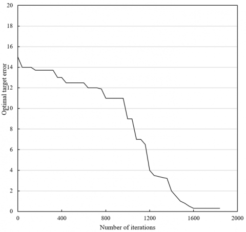
Figure 4 shows the variation curve of the optimal target error during the adaptive PSO. It can be seen that the curve was monotonously decreasing until the optimal value was found or the maximum number tmax of iterations was reached. In actual operation, the desired optimal value was obtained after about 1,500 iterations; after that, the target error remained basically unchanged.
Figure 4. The variation curve of the optimal target error
Next, the proposed PSONN algorithm was compared with the traditional proportional-integral-derivative (PID) control algorithm. Figures 5 and 6 compare the two algorithms in the tracking errors of the angular displacement and displacement at the end of the first and second joints, respectively.
It can be seen that, when the target error of trajectory planning was the same, the PSONN algorithm reduced the tracking error of angular displacement at the end of the first and second joints by 38.79% and 30.48%, respectively, from that of the PID control algorithm; similarly, the PSONN algorithm reduced the tracking error of displacement at the end of the first and second joints by 41.34% and 35.42%, respectively. Overall, our algorithm has a much smaller error than the PID control algorithm in tracking the manipulator trajectory.
Comparing Figures 5(a) and 5(b), both the FNN and PSONN controlled the peak tracking error of angular error within ±1.75. This partially demonstrates the suppression effect of our algorithm on end jitter, which benefits the smooth operation of medical manipulators.
Figure 5. The comparison of the tracking errors of the angular displacement at the end of two joints
Figure 6. The comparison of the tracking errors of displacement at the end of two joints
Figure 7 compares the output torques at the end of two joints under the control of our algorithm and the FNN, respectively. It can be seen that, before being optimized by adaptive PSO algorithm, the FNN control resulted in large fluctuations in the output torques of the first and second joints. After the optimization, the jitter phenomena were obviously mitigated. Therefore, the trajectory of medical manipulator planned by our algorithm can suppress external disturbances as per the needs of the actual objective, improve the ability of jitter suppression, and enhance the positioning accuracy of each joint.
Figure 7. The comparison of the output torques at the end of two joints
Figure 8. The monitored angular velocities of three joints
Figure 8 presents the monitored angular velocities of the three joints of the manipulator. Obviously, the angular velocity of every joint stabilized after 2-3s, indicating that our algorithm can rapidly plan a suitable trajectory for the medical manipulator.
This paper designs a trajectory planning algorithm for medical manipulators by optimizing FNN with an adaptive PSO algorithm. Firstly, a kinetic model was constructed for an n-DOF medical manipulator based on position and posture transforms, and used to construct an FNN for trajectory planning. Then, an adaptive PSO algorithm was developed to suppress the jitter at the end of the medical manipulator, and used to optimize the FNN. The steps of the PSONN algorithm were described in details. Finally, the performance of the proposed PSONN algorithm was tested through experiments on a 3DOF medical manipulator. The experimental results show that our algorithm outperforms the traditional PID control algorithm in tracking error. Moreover, our algorithm was found to have a good ability to suppress the end jitter of the manipulator, enhance jitter suppression and joint positioning accuracy, and achieve a good effect of velocity control.
This work was supported by the Scientific and Technological Research Program of Chongqing Municipal Education Commission (Grant No.: KJQN201903108, KJ1602901), Chongqing College of Electronic Engineering Scientific Research Project (Grant No.: XJZK201809) and Xinxiang Medical University Education and Teaching Reform Research Project (Grant No.: 2017-XYJG-41).
[1] Kamali, K., Joubair, A., Bonev, I. A., Bigras, P. (2016). Elasto-geometrical calibration of an industrial robot under multidirectional external loads using a laser tracker. In 2016 IEEE International Conference on Robotics and Automation (ICRA), pp. 4320-4327. https://doi.org/10.1109/ICRA.2016.7487630
[2] Faulwasser, T., Weber, T., Zometa, P., Findeisen, R. (2016). Implementation of nonlinear model predictive path-following control for an industrial robot. IEEE Transactions on Control Systems Technology, 25(4): 1505-1511. https://doi.org/10.1109/TCST.2016.2601624
[3] Quarta, D., Pogliani, M., Polino, M., Maggi, F., Zanchettin, A.M., Zanero, S. (2017). An experimental security analysis of an industrial robot controller. In 2017 IEEE Symposium on Security and Privacy (SP), pp. 268-286. https://doi.org/10.1109/SP.2017.20
[4] Guillo, M., Dubourg, L. (2016). Impact & improvement of tool deviation in friction stir welding: Weld quality & real-time compensation on an industrial robot. Robotics and Computer-Integrated Manufacturing, 39: 22-31. https://doi.org/10.1016/j.rcim.2015.11.001
[5] Yin, X., Pan, L. (2018). Enhancing trajectory tracking accuracy for industrial robot with robust adaptive control. Robotics and Computer-Integrated Manufacturing, 51: 97-102. https://doi.org/10.1016/j.rcim.2017.11.007
[6] Su, Y.H., Chen, C.Y., Cheng, S.L., Ko, C.H., Young, K.Y. (2018). Development of a 3D AR-based interface for industrial robot manipulators. In 2018 IEEE International Conference on Systems, Man, and Cybernetics (SMC), pp. 1809-1814. https://doi.org/10.1109/SMC.2018.00313
[7] Ayten, K.K., Dumlu, A. (2018). Real-time implementation of sliding mode control technique for two-DOF industrial robotic arm. Iğdır Üniversitesi Fen Bilimleri Enstitüsü Dergisi, 8(4): 77-85.
[8] Koumboulis, F.N. (2018). On the common control design of robotic manipulators carrying different loads. In International Conference on Robotics in Alpe-Adria Danube Region, pp. 416-424. https://doi.org/10.1007/978-3-030-00232-9_44
[9] Sefati, S., Alambeigi, F., Iordachita, I., Taylor, R.H., Armand, M. (2018). On the effect of vibration on shape sensing of continuum manipulators using fiber Bragg gratings. In 2018 International Symposium on Medical Robotics (ISMR), pp. 1-6. https://doi.org/10.1109/ISMR.2018.8333303
[10] Wahrburg, A., Bös, J., Listmann, K. D., Dai, F., Matthias, B., Ding, H. (2017). Motor-current-based estimation of cartesian contact forces and torques for robotic manipulators and its application to force control. IEEE Transactions on Automation Science and Engineering, 15(2): 879-886. https://doi.org/10.1109/TASE.2017.2691136
[11] Capurso, M., Ardakani, M.M.G., Johansson, R., Robertsson, A., Rocco, P. (2017). Sensorless kinesthetic teaching of robotic manipulators assisted by observer-based force control. In 2017 IEEE International Conference on Robotics and Automation (ICRA), pp. 945-950. https://doi.org/10.1109/ICRA.2017.7989115
[12] Yang, T., Yang, Z., Li, T., Liu, S., Wang, Y. (2018). Research on cooperation control of lightweight manipulator. In 2018 37th Chinese Control Conference (CCC), pp. 5498-5503. https://doi.org/10.23919/ChiCC.2018.8482958
[13] Mareczek, J. (2019). Grundlagen der roboter-manipulatoren-band 2: Pfad-und bahnplanung, antriebsauslegung, regelung. Springer Berlin Heidelberg.
[14] Bianco, C.G.L., Raineri, M. (2017). An automatic system for the avoidance of wrist singularities in anthropomorphic manipulators. In 2017 13th IEEE Conference on Automation Science and Engineering (CASE), pp. 1302-1309. https://doi.org/10.1109/COASE.2017.8256280
[15] Navarro, B., Cherubini, A., Fonte, A., Poisson, G., Fraisse, P. (2017). A framework for intuitive collaboration with a mobile manipulator. In 2017 IEEE/RSJ International Conference on Intelligent Robots and Systems (IROS), pp. 6293-6298. https://doi.org/10.1109/IROS.2017.8206532
[16] Mohamed, Z., Khairudin, M., Husain, A.R., Subudhi, B. (2016). Linear matrix inequality-based robust proportional derivative control of a two-link flexible manipulator. Journal of Vibration and Control, 22(5): 1244-1256. https://doi.org/10.1177%2F1077546314536427
[17] Annisa, J., Darus, I.M., Tokhi, M.O., Mohamaddan, S. (2018). Implementation of PID based controller tuned by evolutionary algorithm for double link flexible robotic manipulator. In 2018 International Conference on Computational Approach in Smart Systems Design and Applications (ICASSDA), pp. 1-5. https://doi.org/10.1109/ICASSDA.2018.8477615
[18] Jamali, A., Mat Darus, I.Z., Mohd Samin, P.P., Tokhi, M.O. (2018). Intelligent modeling of double link flexible robotic manipulator using artificial neural network. Journal of Vibroengineering, 20(2): 1021-1034. https://doi.org/10.21595/jve.2017.18575
[19] Annisa, J., Abidin, A.Z., Darus, I.M., Tokhi, M.O. (2018). Controlling the non-parametric modeling of double link flexible robotic manipulator using hybrid PID tuned by P-Type ILA. International Journal of Integrated Engineering, 10(7): 219-232. https://doi.org/10.30880/ijie.2018.10.07.020
[20] Mohammed, A.A., Eltayeb, A. (2018). Dynamics and control of a two-link manipulator using pid and sliding mode control. In 2018 International Conference on Computer, Control, Electrical, and Electronics Engineering (ICCCEEE), pp. 1-5. https://doi.org/10.1109/ICCCEEE.2018.8515795
[21] Bagheri, M., Naseradinmousavi, P., Krstić, M. (2019). Feedback linearization based predictor for time delay control of a high-DOF robot manipulator. Automatica, 108: 108485. https://doi.org/10.1016/j.automatica.2019.06.037
[22] Pizarro-Lerma, A.O., Garcia-Hernandez, R., Santibanez, V., Chin, J.V. (2019). Experimental evaluation of a sectorial fuzzy controller plus adaptive neural network compensation applied to a 2-DOF robot manipulator. IFAC-PapersOnLine, 52(29): 233-238. https://doi.org/10.1016/j.ifacol.2019.12.655
[23] Campisano, F., Remirez, A., Landewee, C.A., Caló, S., Obstein, K., Webster III, R.J., Valdastri, P. (2020). Teleoperation and Contact Detection of a Waterjet-Actuated Soft Continuum Manipulator for Low-Cost Gastroscopy. IEEE Robotics and Automation Letters, 5(4): 6427-6434. https://doi.org/10.1109/LRA.2020.3013900
[24] Wilkening, P., Alambeigi, F., Murphy, R.J., Taylor, R.H., Armand, M. (2017). Development and experimental evaluation of concurrent control of a robotic arm and continuum manipulator for osteolytic lesion treatment. IEEE Robotics and Automation Letters, 2(3): 1625-1631. https://doi.org/10.1109/LRA.2017.2678543
[25] Sefati, S., Murphy, R.J., Alambeigi, F., Pozin, M., Iordachita, I., Taylor, R.H., Armand, M. (2018). FBG-based control of a continuum manipulator interacting with obstacles. In 2018 IEEE/RSJ International Conference on Intelligent Robots and Systems (IROS), pp. 6477-6483. https://doi.org/10.1109/IROS.2018.8594407