Fengqin Zhang
© 2020 IIETA. This article is published by IIETA and is licensed under the CC BY 4.0 license (http://creativecommons.org/licenses/by/4.0/).
OPEN ACCESS
The intelligent adjustment of train operation plan (TOP) is helpful to the efficiency of high-speed rail (HSR) network. This paper attempts to adjust the TOP quickly and intelligently after operation faults, thereby minimize the delay, contain the scope of influence and improve passenger satisfaction. Firstly, the features of a single scheduling section were analyzed based on train flow, highlighting the necessity to design section-specific TOP adjustment strategy and optimization objectives. Next, multiple optimization objectives were designed based on the identified features and passenger satisfaction, and weighted through stochastic intuitionistic fuzzy decision. Finally, the firefly algorithm was improved into chaotic firefly algorithm (CFA) to solve our model. The effectiveness of our algorithm was confirmed through simulation. The research results shed important new light on the TOP adjustment in the HSR network.
high-speed rail (HSR), multi-objective optimization, fuzzy decision, chaotic firefly algorithm (CFA)
High-speed rail (HSR) is an important transport mode that carries a large number of passengers at a fast speed and high frequency. However, operation faults also spread rapidly across the large and complex HSR network. If one train is delayed, the subsequent trains will also operate behind schedule. To restore the normal operations, the train operation plan (TOP) must be adjusted promptly at the centralized traffic control system (CTCS), the brain of the HSR network.
In the event of operation faults, the TOP is generally adjusted in manual mode. During the adjustment, the schedulers need to coordinate between various parties and deal with numerous issues. As a result, the adjusted plan is often inefficient and unreliable, which hinders the automation and intelligence of the HSR network. Against this backdrop, it is an urgent task to adjust the TOP quickly and intelligently at the CTCS in the case of operation faults, thereby minimize the delay, contain the scope of influence and improve passenger satisfaction.
Based on the CTCS, this paper explores the requirements on TOP adjustment in the complex HSR network, and develops a practical TOP adjustment model for a single scheduling section (hereinafter referred to as section) of the HSR network.
The TOP adjustment has long been treated as an optimization problem. For example, Gustavsson [1] constructed a 0-1 mixed integer programming (MIP) model to adjust the TOP in a single section of railway that handles both passenger and cargo traffic. For TOP adjustment, Wen and Li [2] determined the train sequence through tabu search (TS). Chen et al. [3] adjusted the TOP under the full failure of railway section capacity: Considering the uncertainty of failure duration, a two-stage stochastic expectation model with compensation and an incomplete continuous multi-stage decision-making model were established, and solved by branch and bound (BB) algorithm.
Zhang et al. [4] adjusted the TOP under the full failure of HSR section capacity: From the macro level, the train operations in the HSR network were regarded as an event-activity network, a mixed integer route planning model was constructed for TOP adjustment, and the two-stage solution algorithm was adopted to solve the model. Zhang et al. [5] summarized the features of interferences in railway operation, and designed a TOP adjustment strategy through sequence optimization. Focusing on the TOP adjustment of HSR, Wakisaka and Masuyama [6] refined the arrival and departure time of train at the station, and built a HSR TOP adjustment model that simultaneously optimizes arrival time and route; the model aims to minimize the time of train spent in the delayed section under the constraint of the minimum train interval. Cacchiani et al. [7] developed an optimization strategy and plan for the adjustment of the periodic TOP.
Krasemann [8] rescheduled the train sequence for TOP adjustment, created a MIP model to minimize the total delay, and verified the reliability of the model using four heuristic algorithms. Huo and Wu [9] adjusted the TOP for single-track railway with both passenger and cargo traffic, with the aim to minimize the weighted delay of trains. Considering the uncertain conflicts between trains, Zhang et al. [10] adjusted the TOP to minimize the delay of all trains at the terminal station. Nie et al. [11] minimized the deviation of the adjusted TOP from the original TOP in HSR network. Sun et al. [12] optimized punctuality, interval operation time, and freight train operation rate through TOP adjustment. Zhang et al. [13] attempted to minimize the weighted total delay and total number of delayed trains through TOP adjustment.
Xu et al. [14] plotted the discrete event topology of single-track railway, developed a discrete-event TOP adjustment model with maximal overall satisfaction, and proposed the iterative repair algorithm to solve the model. Based on graph theory, Choi et al. [15] constructed a train state diagram for TOP adjustment, expressed train sate in station as a quintuple, and put forward two heuristic search algorithms: node priority search and differential-operator initial time selection based on maximum delay. Zhuang et al. [16] improved the difference algorithm to solve the HSR TOP adjustment model, and proved that the improved algorithm can prevent the premature convergence of the original algorithm. Drawing on adaptive dynamic planning, Chen and Zhou [17] solved the TOP adjustment problem by replacing the cost function with backpropagation neural network (BPNN), and calling the double heuristic dynamic planning algorithm.
The above studies on TOP adjustment have improved the efficiency of railway transport to varied degrees, but most of them focus on a single optimization objective. This paper mainly designs a multi-objective optimization model to adjust the TOP in a single section. In addition to train flow, the optimization objectives also cover multiple indices related to passenger satisfaction.
3.1 Influencing factors of delay
The influencing factors of the delay of a train fall into three categories: human factors, equipment factors and environmental factors. Train delays could be caused by one or several of these factors.
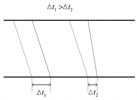
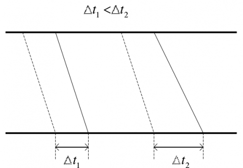
From the perspective of the TOP, a train may fall behind the schedule if there is any change to the interval operation time or stop time. If the delay is small, it could be absorbed by the buffer time on the TOP. Otherwise, the delay will propagate along the railway. The propagation pattern can be divided into attenuated propagation, equivalent propagation and enhanced propagation [18]. The three patterns are respectively illustrated in Figures 1-3, where $\Delta t_{1}$ and $\Delta t_{2}$ are the delays of train 1 and its subsequent train 2, respectively.
Figure 1. Attenuated propagation
Figure 2. Equivalent propagation
Figure 3. Enhanced propagation
3.2 Section features
In the HSR network, each railway is divided into several sections. The trains in the same section are scheduled as one unit. However, it is impossible to make all the trains run on time, if the TOP is interfered by any event. Once a delay occurs, the TOP must be adjusted effectively to curb the delay propagation across the network, protect the safety and efficiency of trains, and ensure the satisfaction of passengers.
The sections differ in location and train flow. Therefore, it is improper to implement the same strategy for TOP adjustment in all sections. For each section, the strategy and optimization objectives of TOP adjustment must be designed in the light of the local features (e.g. train flow). This paper analyzes the features of a single section based on the train flows measured in previous tests.
(1) Train types
Table 1. The statistics on train types in a single section
|
Category |
Type |
Number |
Proportion |
|
Single types |
Start-end |
6 |
17.5% |
|
Arrival-departure |
8 |
||
|
Start-departure |
11 |
||
|
Two types |
Start-end, start-departure |
22 |
55.9% |
|
Arrival-departure, start-departure |
58 |
||
|
Three types |
Start-end, arrival-departure, start-departure |
38 |
26.6% |
Table 2. The statistics on start-end trains
|
Proportion of trains |
Number of sections |
Proportion of sections |
|
x=1 |
6 |
9.37% |
|
0.75£x<1 |
8 |
12.5% |
|
0.5£x<0.75 |
5 |
7.81% |
|
0.25£x<0.5 |
4 |
6.25% |
|
0£x<0.25 |
6 |
9.37% |
|
x=0 |
35 |
54.7% |
Table 3. The statistics on arrival-departure trains
|
Proportion of trains |
Number of sections |
Proportion of sections |
|
x=1 |
8 |
5.93% |
|
0.75£x<1 |
28 |
20.74% |
|
0.5£x<0.75 |
22 |
16.30% |
|
0.25£x<0.5 |
20 |
14.81% |
|
0£x<0.25 |
21 |
15.56% |
|
x=0 |
36 |
26.66% |
Table 4. The statistics on start-departure trains
|
Proportion of trains |
Number of sections |
Proportion of sections |
|
x=1 |
10 |
6.62% |
|
0.75£x<1 |
20 |
13.24% |
|
0.5£x<0.75 |
27 |
17.88% |
|
0.25£x<0.5 |
25 |
16.56% |
|
0£x<0.25 |
36 |
23.85% |
|
x=0 |
33 |
21.85% |
As shown in Table 1, more than 82% of the sections have two or more types of trains. Only a few sections contain a single type of trains. The statistics on different types of trains are given in Tables 2-4.
(2) Trains speeds
Based on operating speed, the trains can be categorized as high-speed electric multiple unit (EMU) train (train code: G), EMU train (train code: D), and intercity EMU train (train code: C).
Table 5. The statistics on train speeds in a single section
|
Category |
Type |
Number |
Proportion |
|
One type |
G |
2 |
23.67% |
|
D |
32 |
||
|
C |
6 |
||
|
Two types |
G and D |
82 |
53.84% |
|
G and C |
4 |
||
|
D and C |
5 |
||
|
Three types |
G, D and C |
38 |
22.49% |
As shown in Table 5, a section may contain EMU trains operating at the same or different speeds. Some sections have a single type of EMU trains, while some have multiple types of EMU trains.
(3) Operation areas
In terms of operation area, the trains could operate within the current section, across sections of the same railway bureau, and across those of different railway bureaus.
Table 6. The statistics on operation areas of trains in a single section
|
Category |
Type |
Number |
Proportion |
|
One type |
Operation in the current section |
4 |
18.98% |
|
Cross-section operation of the same bureau |
10 |
||
|
Cross-bureau operation |
12 |
||
|
Two types |
Operation in the current section + cross- section operation of the same bureau |
8 |
54.01% |
|
Operation in the current section + cross-bureau operation |
10 |
||
|
Cross-section operation of the same bureau + cross-bureau operation |
56 |
|
|
|
Three types |
Operation in the current section + cross-section operation of the same bureau + cross-bureau operation |
37 |
27.01% |
As shown in Table 6, a section may contain trains with various operation areas. Some sections have a single type of trains, while some have multiple types of trains.
(4) The number of adjacent sections in the train direction
Table 7. The number of adjacent sections in the train direction
|
Number of adjacent sections |
Number of sections |
Proportion of sections |
|
0 |
6 |
4.44% |
|
1 |
30 |
22.22% |
|
2 |
32 |
23.7% |
|
3 |
33 |
24.44% |
|
4 |
20 |
14.82% |
|
5 |
12 |
8.89% |
|
6 |
2 |
1.49% |
As shown in Table 7, the trains running in one of the first six sections only operate in the current section, because there is zero adjacent section in the train direction.
The above analysis shows that the TOP of each section should be adjusted differently according to the its location in the HSR network, the features of train flow, the type of interference event and the features of passenger flow.
4.1 Constraints
For single-section TOP adjustment, the multi-objective optimization is subjected to the following constraints:
(1) The stop time of the train at the station should not be shorter than the minimum stop time of the train: $T_{r_{i}, u_{j}}^{d}-T_{r_{i}, u_{j}}^{a} \geq t_{r_{i}, u_{j}}^{\min }$.
where, $T_{r_{i}, u_{j}}^{d}$ and $T_{r_{i}}^{a} u_{j}$ are the departure time and arrival time of train line $r_{i}$ at station $u_{j},$ respectively; $t_{r i, u j}^{m i n}$ is the minimum stop time of the train.
(2) The time interval of train arrival at station should satisfy the following constraint:
If If $B_{r_{i}, u_{j}}^{A} \cap B_{{{r}_{i'}},{{u}_{j}}}^{A} \neq \emptyset,$ then $\left|T_{r_{i} u_{j}}^{A}-T_{{{r}_{i'}},{{u}_{j}}}^{A}, u_{j}\right| \geq t_{u_{j}}^{A A}$.
where, $B_{r_{i}, u_{j}}^{A}$ and $T_{r_{i}, u_{j}}^{A}$ are the arriving route and arriving time of train line $r_{i}$ at station $u_{j}$, respectively.
(3) The time interval of train departure at station should satisfy the following constraint:
If $B_{r_{i}, u_{j}}^{D} \cap B_{{{r}_{i'}},{{u}_{j}}}^{D} \neq \emptyset,$ then $\left|T_{r_{i}, u_{j}}^{D}-T_{r_{i}^{\prime}}^{D}, u_{j}\right| \geq t_{u_{j}}^{D D}$.
where, $B_{r_{i}, u_{j}}^{D}$ and $T_{r_{i}, u_{j}}^{D}$ are the departure route and departure time of train line $r_{i}$ at station $u_{j}$, respectively.
(4) The time intervals of train arrival and departure at station should satisfy the following constraints:
If $B_{r_{i}, u_{j}}^{D} \cap B_{{{r}_{i'}},{{u}_{j}}}^{A} \neq \varnothing$, then $T_{r_{i}, u_{j}}^{D}-T_{{{r}_{i'}},{{u}_{j}}}^{A}, \geq t_{u_{j}}^{A D}$ or $T_{{{r}_{i'}},{{u}_{j}}}^{A}-T_{r_{i}, u_{j}}^{D}, \geq t_{u_{j}}^{D A}$.
If $B_{r_{i}, u_{j}}^{A} \cap B_{{{r}_{i'}},{{u}_{j}}}^{D} \neq \varnothing$, then $T_{{{r}_{i'}},{{u}_{j}}}^{D} \geq t_{u_{j}}^{A D}$ or $T_{r_{i}, u_{j}}^{A}-T_{{{r}_{i'}},{{u}_{j}}}^{D} \geq t_{u_{j}}^{D A}$.
(5) If the train line $r_{i}$ has a train connection at station $u_{j}$, the minimum connection time should satisfy the following constraint:
If $r_{i} \in c_{k}, c_{k}=\left\{r_{i}, r_{i'}, u_{j}\right\}$, then $T_{{{r}_{i'}},{{u}_{j}}}^{D}-T_{r_{i}, u_{j}}^{A} \geq t_{c_{k}}^{\min }$.
If $r_{i} \in c_{k}, c_{k}=\left\{r_{i'}, r_{i}, u_{j}\right\}$, then $T_{r_{i}, u_{j}}^{D}-T_{{{r}_{i'}},{{u}_{j}}}^{A}, u_{j} \geq t_{c_{k}}^{\min }$.
(6) The arrival time of train at departure station should satisfy the following constraint:
If $u_{j}=u_{r_{i}}^{0},$ then $T_{r_{i}, u_{j}}^{A}=T_{r_{i}, u_{j}}^{D}$.
(7) The departure time of train at terminal station should satisfy the following constraint:
If $u_{j}=u_{r_{i}}^{e},$ then $T_{r_{i}, u_{j}}^{D}=T_{r_{i}, u_{j}}^{A}$.
4.2 Objective functions
Two sets of objective functions were established for single-section TOP adjustment: those based on train flow features and those based on passenger satisfaction.
There are four objective functions based on train flow features:
(1) Minimum delay at station
$o b_{1}^{T}=\min \sum_{i=1}^{s} \sum_{j=1}^{t}\left(w_{r_{i}, u_{j}}^{d-A} \cdot t_{r_{i}, u_{j}}^{d-A}+w_{r_{i}, u_{j}}^{d-D} \cdot t_{r_{i}, u_{j}}^{d-D}\right)$
where, $w_{r_{i}, u_{j}}^{d-A}$ is the weight of train line $r_{i}$ arriving delay at station $u_{j} ; w_{r_{i}, u_{j}}^{d-D}$ is the weight of train line $r_{i}$ departure delay at station $u_{j}$
(2) Minimum departure delay of the departure train in the current section at the departure station:
$o b_{2}^{T}=\min \sum_{i=1}^{s} t_{r_{i}, w_{r_{i}}^{o}}^{d-A}\cdot t_{r_{i}, u_{r_{i}}^{o}}^{d-A}$
(3) Minimum arrival time of the terminal train in the current section at the terminal station:
$o b_{3}^{T}=\min \sum_{i=1}^{s} w_{r_{i}, u_{r_{i}}^{e}}^{d-A} \cdot t_{r_{i}, u_{r_{i}}^{e}}^{d-A}$
(4) Minimum number of delayed trains
$o b_{4}^{T}=\min \sum_{i=1}^{s} T_{r_{i}}^{d e l a y}$
There are two objective functions based on passenger satisfaction:
(1) Minimum delay at station for passenger satisfaction
$o b_{1}^{P}=\sum_{i=1}^{s} \sum_{j=1}^{t}\left(w_{r_{i}, u_{j}}^{S 1} \cdot\left(t_{r_{i}, u_{j}}^{d-A}+t_{r_{i}, u_{j}}^{d-D}\right)\right.$
(2) Minimum delay at station for transfer passengers’ satisfaction
$o b_{2}^{P}=\sum_{i=1}^{s} \sum_{j=1}^{t} w_{r_{i}, u_{j}}^{S 2} \cdot t_{r_{i}, u_{j}}^{d-A}$
The robustness of the overall objective function depends on the weight of each objective function. The weighting of objective functions is a multi-attribute decision-making problem with high fuzziness and uncertainty. The fuzzy, uncertain problem can be solved satisfactorily with intuitionistic fuzzy sets [19]. Therefore, the stochastic intuitionistic fuzzy decision-making algorithm was adopted to determine the weight of each index in the overall objective function.
The two sets of weighted objective function were integrated into an overall objective function for the multi-objective optimization:
$o b=\rho_{1}^{T} o b_{1}^{T}+\rho_{2}^{T} o b_{2}^{T}+\rho_{3}^{T} o b_{3}^{T}+\rho_{4}^{T} o b_{4}^{T}+\rho_{5}^{T} o b_{1}^{P}$
$+\rho_{6}^{T} o b_{2}^{P}$
4.3 Model solving with the CFA
To solve our TOP adjustment model, the basic firefly algorithm is improved into the CFA through the logical self-mapping below:
$y_{n+1}=f\left(\mu, y_{n}\right)=1-\mu y_{n}^{2}$ (1)
where, $n=0,1,2, \ldots, \infty,-1<y_{n}<1 ; \mu$ is the control parameter.
Based on logical self-mapping, the CFA optimization process is as follows:
(1) The solution of firefly algorithm is mapped to [-1, 1]:
$L_{d}=2 * \frac{x_{d}-a_{d}}{b_{d}-a_{d}}-1$ (2)
where, $x_{d}$ is the position of firefly i in the d-dimensional space; $a_{d}$ and $b_{d}$ are the lower and upper search bounds of each variable, respectively.
(2) The generated chaotic variable is introduced into the optimization model, and the new chaotic variable is obtained using the chaos operator:
$L_{n+1, d}=1-2 L_{n, d}^{2}$ (3)
where, $d=1,2, \ldots, D ; n=0,1,2, \ldots, \infty ;-1<L_{n, d}<1$.
(3) The obtained chaotic variable sequence is converted to the original solution space:
$y_{d}^{\prime}=\frac{\left(b_{d}-a_{d}\right) * L_{d}+\left(b_{d}+a_{d}\right)}{2}$ (4)
where, $d=1,2, \ldots, D ; a_{d}$ and $b_{d}$ are the lower and upper search bounds of each variable, respectively.
If the current position of a firefly is better than the original position, then the original position of that firefly should be replaced by the current position. Otherwise, the algorithm continues until meeting the termination condition.
In each round, if all fireflies are optimized by the chaos operator, the algorithm will become more accurate. However, the improved accuracy comes at the cost of a longer runtime. To improve the algorithm efficiency, a few fireflies should be selected for chaotic optimization. Here, the search space is adjusted dynamically to change the upper and lower search bounds in each dimension. The upper and lower search bounds can be defined respectively as:
$y_{\min , d}=\max \left\{y_{\min , d}, y_{g, d}-\rho *\left(y_{\max , d}-y_{\min , d}\right)\right\}$ (5)
$\begin{aligned} y_{\max , d}=\min \left\{y_{\max , d}, y_{g, d}+\rho\right.& \\\left.*\left(y_{\max , d}-y_{\min , d}\right)\right\} \end{aligned}$ (6)
where, $y_{g, d}$ is the value of the current optimal solution in the d-dimensional space; $\rho$ is the transform factor.
The workflow of the CFA based on logical self-mapping is explained as follows:
Step 1. Initialize the number and positions of fireflies based on the arrival time and departure time of the target train at the station.
Step 2. Derive the maximum brightness from the initial positions of fireflies.
Step 3. Calculate the relative brightness and attractiveness of each firefly.
Step 4. Update the position of each firefly.
Step 5. Select the best s% of fireflies for chaotic optimization with logical self-mapping and dynamic transform of the search space, and replace the worst s% fireflies with the s% newly generated fireflies.
Step 6. Recalculate the brightness of each firefly after the position update.
Step 7. Output the optimal solution if the maximum number of iterations is reached or the search accuracy is as required; otherwise, jump to Step 3 for iterative search.
To verify the effectiveness of the CFA in solving our multi-objective optimization problem, four performance metrics were selected: generation distance (GD), convergence ($\gamma$), space (SP) and dispersion ($\Delta$). The four metrics can be respectively defined as follows:
$G D=\frac{\sqrt{\Sigma_{i=1}^{n} p_{i}^{2}}}{n}$
where, n is the number of Pareto solutions obtained by the algorithm; $p_{i}$ is the shortest distance between the i-th solution and the real Pareto solution.
$\gamma=\frac{1}{|P|} \sum_{i=1}^{|P|} \min _{i \leq j \leq\left|p^{*}\right|}\left(\left|a_{i}-p_{j}\right|\right)$
where, $p^{*}$ is the real Pareto solution; P is the Pareto solutions obtained by the algorithm.
$S P=\sqrt{\frac{1}{n-1} \sum_{i=1}^{n}\left(\bar{p}-p_{i}\right)^{2}}$
where, $p_{i}$ is the shortest distance between the i-th solution and the real Pareto solution; $\bar{p}$ is the mean of all $p_{i}$ values; n is the number of Pareto solutions.
$\Delta=\frac{p_{f}+p_{d}+\sum_{i}^{n-1}\left|p_{i}-\bar{p}\right|}{p_{f}+p_{d}+(n-1) \bar{p}}$
where, $p_{f}$ and $p_{d}$ are the distances between the boundary solution and the corresponding extreme solutions of the Pareto solution set.
The population size is an important factor to algorithm performance. An excessively small population will affect the convergence and diversity of the algorithm. Table 8 lists the mean values of the four metrics at different population sizes. Obviously, most of the metrics were optimized when the population had ten fireflies.
Hence, the proposed CFA was compared with the multiple objective particle swarm optimization (MOPSO) algorithm [20] in solving our TOP adjustment model at the population size of 10. The metrics of the two algorithms are recorded in Tables 9 and 10, respectively.
Table 8. The mean values of the four metrics at different population sizes
|
Population size |
GD |
γ |
SP |
∆ |
Number of Pareto optimal solutions |
|
2 |
0.0172 |
0.082 |
0.021 |
0.789 |
43.2 |
|
5 |
0.0171 |
0.097 |
0.015 |
0.772 |
38.6 |
|
10 |
0.0147 |
0.069 |
0.013 |
0.739 |
46.8 |
|
20 |
0.0155 |
0.073 |
0.028 |
0.863 |
35.8 |
Table 9. The metrics of the MOPSO algorithm
|
|
GD |
γ |
SP |
∆ |
Number of Pareto optimal solutions |
|
Mean |
0.025 |
0.109 |
0.037 |
0.787 |
26.6 |
|
Mean-square deviation |
0.0026 |
0.0038 |
0.0019 |
0.0178 |
- |
|
Maximum |
0.065 |
0.247 |
0.236 |
1.271 |
51 |
|
Minimum |
0.005 |
0.028 |
0.008 |
0.543 |
10 |
Table 10. The metrics of the CFA
|
|
GD |
γ |
SP |
∆ |
Number of Pareto optimal solutions |
|
Mean |
0.014 |
0.086 |
0.018 |
0.749 |
47.9 |
|
Mean-square deviation |
0.0000 |
0.0012 |
0.0000 |
0.0008 |
- |
|
Maximum |
0.032 |
0.163 |
0.447 |
0.912 |
87 |
|
Minimum |
0.003 |
0.026 |
0.005 |
0.493 |
15 |
From Tables 9 and 10, it can be seen that the CFA outperformed the MOPSO algorithm in most of the metrics. Compared with the MOPSO algorithm, our algorithm converges quickly to a large set of diverse Pareto optimal solutions.
This paper probes deep into the TOP adjustment in the complex HSR network, aiming to restore the normal operations of trains quickly and intelligently after the occurrence of faults (e.g. delay). The features of a single section were analyzed in details based on train flow. Based on these features and passenger satisfaction, a TOP adjustment model was established with multiple optimization objectives, each of which has a unique weight. Next, the weighting of the objectives was taken as a multi-attribute decision-making problem, and completed through stochastic intuitionistic fuzzy decision-making. After that, the firefly algorithm was improved into the CFA to solve our model. Simulation results show that the CFA can effectively solve our TOP adjustment model. Our research provides a realistic strategy to tackle the delays in the HSR network.
[1] Gustavsson, E. (2015). Scheduling tamping operations on railway tracks using mixed integer linear programming. EURO Journal on Transportation and Logistics, 4(1): 97-112. https://doi.org/10.1007/s13676-014-0067-z
[2] Wen, C., Li, B. (2013). Train operation adjustment based on conflict resolution for high-speed rail. Journal of Transportation Security, 6(1): 77-87. https://doi.org/10.1007/s12198-012-0104-9
[3] Chen, Y.J., Zhou, L.S., Yu, J.A. (2013). Study on ordinal optimization strategies of train operation adjustment plan of heavy haul railway. Journal of the China Railway Society, 35(1): 1-7.
[4] Zhang, L., Qin, Y., Meng, X., Wang, L., Zhu, T. (2016). MPSO-based model of train operation adjustment. Procedia Engineering, 137, 114-123. https://doi.org/10.1016/j.proeng.2016.01.241
[5] Zhang, J., Yang, H., Wei, Y., Shang, P. (2016). The empty wagons adjustment algorithm of Chinese heavy-haul railway. Chaos, Solitons & Fractals, 89: 91-99. https://doi.org/10.1016/j.chaos.2015.10.011
[6] Wakisaka, K., Masuyama, S. (2012). Automatic construction of train arrival and departure schedules at terminal stations. Journal of Advanced Mechanical Design, Systems, and Manufacturing, 6(5): 590-599. https://doi.org/10.1299/jamdsm.6.590
[7] Cacchiani, V., Galli, L., Toth, P. (2015). A tutorial on non-periodic train timetabling and platforming problems. Euro Journal on Transportation and logistics, 4(3): 285-320. https://doi.org/10.1007/s13676-014-0046-4
[8] Krasemann, J.T. (2012). Design of an effective algorithm for fast response to the re-scheduling of railway traffic during disturbances. Transportation Research Part C: Emerging Technologies, 20(1): 62-78. https://doi.org/10.1016/j.trc.2010.12.004
[9] Huo, J.W., Wu, J.J. (2012). Modeling and solving of balance-based single track railway mixed passenger and freight trains rescheduling. Shandong Science, 25(3): 12-17.
[10] Zhang, T., Li, D., Qiao, Y. (2018). Comprehensive optimization of urban rail transit timetable by minimizing total travel times under time-dependent passenger demand and congested conditions. Applied Mathematical Modelling, 58: 421-446. https://doi.org/10.1016/j.apm.2018.02.013
[11] Nie, L., Zhao, P., Yang, H., Hu, A.Z. (2001). Study on motor trainset operation in high speed railway. Journal of the China Railway Society, 23(3): 1-7.
[12] Sun, Y., Cao, C., Wu, C. (2014). Multi-objective optimization of train routing problem combined with train scheduling on a high-speed railway network. Transportation Research Part C: Emerging Technologies, 44: 1-20. https://doi.org/10.1016/j.trc.2014.02.023
[13] Zhang, C.Y., Chen, D., Yin, J., Chen, L. (2017). A flexible and robust train operation model based on expert knowledge and online adjustment. International Journal of Wavelets, Multiresolution and Information Processing, 15(03): 1750023. https://doi.org/10.1142/S0219691317500230
[14] Xu, X., Li, K., Yang, L. (2016). Rescheduling subway trains by a discrete event model considering service balance performance. Applied Mathematical Modelling, 40(2): 1446-1466. https://doi.org/10.1016/j.apm.2015.06.031
[15] Choi, J., Kim, H.U., Yang, S., Kim, T. (2018). Numerical analysis of particle concentration around the air-inlet of a train in a tunnel by using a discrete phase model. Journal of Mechanical Science and Technology, 32(2): 717-722. https://doi.org/10.1007/s12206-018-0120-6
[16] Zhuang, H., Feng, L., Wen, C., Peng, Q., Tang, Q. (2016). High-speed railway train timetable conflict prediction based on fuzzy temporal knowledge reasoning. Engineering, 2(3): 366-373. https://doi.org/10.1016/J.ENG.2016.03.019
[17] Chen, Y.J., Zhou, L.S. (2010). Study on train operation adjustment algorithm based on ordinal optimization. Journal of the China Railway Society, 32(3): 1-8.
[18] Sun, G., Bin, S. (2018). A new opinion leaders detecting algorithm in multi-relationship online social networks. Multimedia Tools and Applications, 77(4): 4295-4307. https://doi.org/10.1007/s11042-017-4766-y
[19] Deb, K., Banerjee, S., Chatterjee, R.P., Das, A., Bag, R. (2019). Educational website ranking using fuzzy logic and k-means clustering based hybrid method. Ingénierie des Systèmes d’Information, 24(5): 497-506. https://doi.org/10.18280/isi.240506
[20] Bo, Z., Cao, Y.J. (2005). Multiple objective particle swarm optimization technique for economic load dispatch. Journal of Zhejiang University-Science A, 6(5): 420-427. https://doi.org/10.1631/jzus.2005.A0420