Aboura Benmansour Souhila* | Demim Fethi | Omari Abdelhafid
OPEN ACCESS
Hyper dynamic manipulation is an emerging control method that simulates the high-speed swing motions of golfer. This paper mainly designs a sliding mode observer for hyper dynamic manipulation, aiming to optimize the trajectory planning for robots. A golf swing robot with two actuated joints and mechanical stoppers was taken as the research object. To optimize the robot trajectory, the authors designed a control strategy with computed torque, and applied it to trajectory monitoring and simulation. In addition, a robust sliding mode observer was developed to estimate the states of the computed torque control, and eliminate the impact of modeling errors and uncertainties. Finally, the sliding mode observer based on computed torque control was proved effective and robust in optimizing the robot trajectory through numerical simulation.
computed torque, golf swing robot, hyper dynamic manipulation, sliding mode observer, stability
Recently we have witnessed an increasing interest for a hyper dynamic manipulation which is defined as a highly skillful manipulation with high motion specifications. As a case study, we consider golf swing robot which has been investigated in recent years to simulate the ultra-high-speed swing motions of professional golfers in order to evaluate the performance of golf clubs and golf balls [1-5].
Currently, there are various golf swing robots on the market with two or more joints, which are attached by gears and belts with a completely interrelated movement. In addition, the joints are always controlled according to the specified head speed during oscillation. Therefore, although the user can modify the initial posture and swing robot speed, the swing movement cannot be adapted depending on the dynamic characteristics of individual golf clubs.
This kind of robot has become an interesting and challenging topic. The researches of Suziki et al. [6] and Ming et al. [7-8] have worked on a mathematic model that has been contributed to the under-actuated manipulator. In these studies, wrist joint was considered as a passive joint containing only a brake mechanism that emulates the wrist cocking action of golfer. On the other hand, Aicardi [9] considered a triple pendulum robotic model for the analysis of the golf swing. In the same context, Hoshino et al. [10] developed a robot which has two joints, a rigid link and a flexible link that is a golf club. They discussed the vibration control problem of their golf swing robot and proposed an optimal control scheme using a state observer that considered a disturbance to suppress the vibration. Hunt and Wiens [11] built a parallel arm robot with five joints. The advantage of this model is that gives a much more realistic and accurate reflection of a human’s golf swings. However, this makes the prototype more expensive and heavier. They use more energy because of in them architectures need five actuators. To avoid these disadvantages, Xu et al. [12] proposed a model with two degrees of freedom that consists of two actuated joints (wrist and shoulder), two rigid links (arm and club) and mechanical stoppers. Compared to the conventional manipulators, this model is inspired by the human ingenious structure [13]: the wrist joint is lighter and less powerful than the shoulder joint. However, to improve dynamic performances, human intervention in this case, can transfer the power/torque from a heavier and stronger body part to the end of the arm, during a dynamic manipulation. In this context, this torque is called dynamic coupled driving.
To validate this original vision in this study, the golf swing robot which is considered consists of two joints: shoulder joint with a powerful direct-drive motor and wrist joint with a small direct-drive motor. The latter is limited by mechanical stoppers in order to reproduce the human’s wrist function. It is necessary to use dynamically coupled driving to realize high-speed swing motions. The robot's motion is considered as an extension of hyper dynamic manipulation and it is generated using multi-objective optimization with strong nonlinear constraints and multiple boundary conditions [14-17].
The golf swing motion control outstanding interests many researchers. For example, Xu et al. [14] applied a PID controller to reduce the robot's tracking error. Studies from Xu et al. [18] and Xu et al. [19] reported that an energy controller is adopted to realize a specified hitting speed at the impact position in the swing. Meanwhile, for the stopping problem that arises from follow-through, a PD control and PD plus Gravity and Coupling Torque Compensation (PGCTC) feedback control taken into smoothly slow down and stop swinging at a specified finish position. Others, conventional controllers devoted to robotics have also been tested [20]. However, not all of these conventional controllers can overcome the internal and external disturbances, which influence the behavior of robot . In our previous work [20], a sliding mode controller, a backstepping controller and a hybrid controller were applied to the robot which combines sliding mode with backstepping are proposed. Nevertheless, these control laws are based on complete state feedback. However, in many practical situations, the joint angular velocities are obtained either by differentiating the measured joint angular positions or through tachymeter. In both cases, the velocity signal is contaminated by the noise. This can reduce the dynamic performance of closed-loop robot systems and influence its stability. To overcome this problem, the $H_{\infty}$ observer was used to estimate joint angular velocities [21].
In this paper, the computed torque controller based on a robust sliding mode observer is proposed to improve the robustness of the system with respect to the external disturbances and uncertainties.
The remainder of this paper is organized as follows: First, the robot’s mechanism and model are introduced in Section 2. Secondly, the design of the sliding mode observer is described in Section 3. In Section 4, this observer is combined with a computed torque controller. Then, simulation tests of the proposed approach are presented in Section 5. Finally, Section 6 concludes the paper results and gives some future works.
2.1 Prototype of the robot
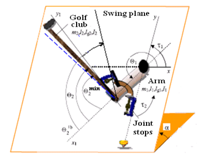
In this section, we consider a golf swing robot, consisting of two joints and mechanical joint stoppers, developed by Ming and his team [13]. This robot has an ingenious structure like the human arm. So, the first joint (shoulder) is driven by a high-power direct-drive motor, which is suitable for hyper dynamic manipulation, and the second joint (wrist) is driven by light and low-power direct-drive motor. Figure 1(a) shows the robot’s prototype, and Table 1 [14] gives it link parameters. The rotation range of each joint I, (i=1, 2), is limited and it is given by Eq. (1).
$\theta _{i}^{\min }\le {{\theta }_{i}}\le \theta _{i}^{\max },_{{}}^{{}}(i=1,2)$ (1)
Table 1. Parameters of the robot
|
Parameter |
Symbol |
Value |
|
Masse of arm (kg) |
m1 |
4.5 |
|
Moment of arm inertia (kg.m2) |
I1 |
1.27 |
|
Length of arm (m) |
l1 |
0.4 |
|
Location of arm centroid (m) |
lg1 |
0.1333 |
|
Mass of club (kg) |
m2 |
1.24 |
|
Moment of club inertia (kgm2) |
I2 |
0.00033 |
|
Length of club (m) |
l2 |
0.95 |
|
Location of club centroid (m) |
lg2 |
0.3167 |
|
Maximum torque of joint 1 (N.m) |
\[\tau _{1}^{\max }\] |
110 |
|
Minimum torque of joint 1 (N.m) |
\[\tau _{1}^{\min }\] |
100 |
|
Maximum torque of joint 2 (N.m) |
\[\tau _{2}^{\max }\] |
11 |
|
Minimum torque of joint 2 (N.m) |
\[\tau _{2}^{\min }\] |
10 |
Consequently, the joint stops working rang is 20 degrees. This constraint is written as:
$\left\{ \begin{matrix} \theta _{2}^{lb}\le {{\theta }_{2}}\le \theta _{2}^{\min } \\ \theta _{2}^{\max }\le {{\theta }_{2}}\le \theta _{2}^{ub} \\\end{matrix} \right.$ (2)
(a) Model of robot
(b) Joint stop
Figure 1. Prototype of the golf swing robot
where,
$\left\{ \begin{matrix} \theta _{2}^{lb}(\deg )=\theta _{2}^{\min }(\deg )+20(\deg ) \\ \theta _{2}^{ub}(\deg )=\theta _{2}^{\max }(\deg )-20(\deg ) \\\end{matrix} \right.$ (3)
The active torques saturations of actuators, given by Eq. (4), are important constraints for the realization of the ingenious structure in a hyper dynamic manipulation.
$\forall t\in [{{t}_{0}},{{t}_{f}}],\tau _{i}^{\min }\le {{\tau }_{i}}(t)\le \tau _{i}^{\max },(i=1,2)$ (4)
2.2 Golf swing motion
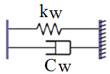
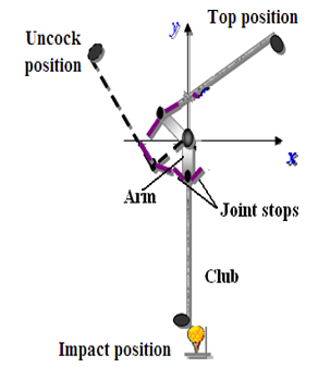
The whole golf swing motion can be divided into three primary phases [15], as shown in Figure 2.
2.2.1 Backswing phase (from the initial position to top position)
In the begging of this phase, both the club and the arm are vertically downward. Then the club is taken back from the initial position to its top position.
2.2.2 Downswing phase (from the top position to impact position)
This phase reflects the hyper dynamic manipulation. The club is swung down from the top position to the impact position to hit a golf ball.
2.2.3 Follow through phase (from the impact position to final position)
After impacting the golf ball, the robot is slowed down and finally stopped.
(a) Backswing phase
(b) Dowswing phase
(c) Follow through phase
Figure 2. Mechanism of golf swing robot
2.3 Dynamic model of the robot
For $(i=1,2)$, a dynamic model of the robot is derived using Lagrange approach, Eq. (5).
${{\Gamma }_{1,2}}=M(\theta )\ddot{\theta }+N(\theta ,\dot{\theta })\dot{\theta }+G(\theta )$ (5)
The mathematical model corresponding to the passive torque generated by joint stops is presented as follows:
$\left\{ \begin{matrix}\tau _{2passif}^{_{\min }}={{k}_{w}}\left( {{\theta }_{2}}-\theta _{2}^{\min } \right)-{{c}_{w}}{{{\dot{\theta }}}_{2}} \\\tau _{2passif}^{_{\max }}={{k}_{w}}\left( {{\theta }_{2}}-\theta _{2}^{\max } \right)-{{c}_{w}}{{{\dot{\theta }}}_{2}} \\\end{matrix} \right.$ (6)
The torque of joint 2 is shown by the Eq. (7):
$\tau {}_{2}(t)=\left\{ \begin{matrix}{{\tau }_{2actif}}(t)+\tau _{2passif}^{_{\min }} \\{{\tau }_{2actif}}(t) \\{{\tau }_{2actif}}(t)+\tau _{2passif}^{_{\max }} \\\end{matrix}\begin{matrix}{{\theta }_{2}}\in \left[ \theta _{2}^{_{lb}},\theta _{2}^{\min } \right) \\{{\theta }_{2}}\in \left[\theta _{2}^{\min },\theta _{2}^{\max } \right] \\{{\theta }_{2}}\in \left( \theta _{2}^{\max },\theta _{2}^{_{ub}} \right] \\\end{matrix} \right.$ (7)
The golf swing robot model is the non-linear and dynamically coupled system.
The main objective of the observer is to estimate the angular velocities using the measurements of the angular positions, assumed to be accessible, while ensuring convergence of the observation error to zero. This observer must also prove its robustness against external disturbances and system’s uncertainties. The estimation is carried out using a robust sliding mode observer.
3.1 State-space representation
The proposed observer is based on a state-space observable form of the Eq. (5), is given by:
$\dot{x}=M^{-1}(x)\left[\Gamma_{1,2}-N(x, \dot{x}) \dot{x}-G(x)\right]$ (8)
where, $x=\left[\begin{array}{ll}{x_{1}} & {x_{2}}\end{array}\right]^{T}$ : represents the state vector of system, with $x_{1}=\left[\begin{array}{ll}{\theta_{1}} & {\theta_{2}}\end{array}\right]^{T}$ , $x_{2}=\left[\begin{array}{ll}{\dot{\theta}_{1}} & {\dot{\theta}_{2}}\end{array}\right]^{T}$ .
$\Gamma=\left[\begin{array}{ll}{\tau_{1}} & {\tau_{2}}\end{array}\right]^{T}$ : defines the input control.
In the dynamic system, Eq. (8) can be rewritten as follows:
$\left\{\begin{array}{l}{\dot{x}_{1}=x_{2}} \\ {\dot{x}_{2}=-M^{-1}\left(x_{1}\right)\left[N\left(x_{1}, x_{2}\right) x_{2}+G\left(x_{1}\right)-\Gamma_{1,2}\right]}\end{array}\right.$ (9)
For simplicity, we can define:
$\beta\left(x_{1}, x_{2}\right)=-M^{-1}\left(x_{1}\right)\left[N\left(x_{1}, x_{2}\right) x_{2}+G\left(x_{1}\right)\right]$ (10)
Then, the system which is given by Eq. (9), can be written as:
$\left\{\begin{array}{l}{\dot{x}_{1}=x_{2}} \\ {\dot{x}_{2}=\beta\left(x_{1}, x_{2}\right)+M^{-1}\left(x_{1}\right) \Gamma_{1,2}} \\ {y=x_{1}}\end{array}\right.$ (11)
$y=\left[\theta_{1} \theta_{2}\right]^{\tau}$ : represents the measurement outputs vector.
3.2 Sliding mode observer
From the synthesis of the observer, we see that our system, given by Eq. (11), is in a class of triangular systems disrupted, with x2 system states supposed inaccessible to measurement, which will allow us to develop our sliding mode observer [22].
The proposed observer ensures convergence of the state observation error $e_{o b s}=(\hat{x}-x)$ and has the following state-space model:
$\left\{\begin{array}{c}{\dot{\hat{x}}_{1}=\hat{x}_{2}-\Lambda_{1} \operatorname{sign}\left(\bar{x}_{1}\right)} \\ {\dot{\hat{x}}_{2}=\beta\left(y, \hat{x}_{2}\right)+M^{-1}\left(x_{1}\right) \Gamma_{1,2}-\Lambda_{2} \operatorname{sign}\left(\bar{x}_{1}\right)} \\ {\hat{y}=\hat{x}_{1}}\end{array}\right.$ (12)
where,
$\bar{x}_{1}=\hat{x}_{1}-x$
$\Lambda_{1}$ and $\Lambda_{2}$ : are defined as:
$\Lambda_{1}=\left(\begin{array}{cc}{\lambda_{1}} & {0} \\ {0} & {\lambda_{1}}\end{array}\right), \quad \Lambda_{2}=\left(\begin{array}{cc}{\lambda_{2}} & {0} \\ {0} & {\lambda_{2}}\end{array}\right)$ (13)
3.2.1 Definition of coefficient matrices
The observation error $e_{o b s}$ is given as the difference between the process output $\mathcal{Y}$ and the estimated output $\hat{y}$ .
$e_{o b s}=\hat{y}-y=\hat{x}_{1}-x_{1}$ (14)
Next, consider the following definition and by introducing the Eq. (15), the state estimation errors are presented as:
$\left\{\begin{array}{l}{\bar{x}_{1}=\hat{x}_{1}-x_{1}} \\ {\bar{x}_{2}=\hat{x}_{2}-x_{2}}\end{array}\right.$ (15)
Finally, the system error equation can be expressed as follows:
$\left\{\begin{aligned} \dot{\bar{x}}_{1} &=\bar{x}_{2}-\Lambda_{1} \operatorname{sign}\left(\bar{x}_{1}\right) \\ \dot{\bar{x}}_{2} &=\Delta \beta\left(y, \hat{x}_{2}, x_{2}\right)-\Lambda_{2} \operatorname{sign}\left(\bar{x}_{1}\right) \end{aligned}\right.$ (16)
where, $\Delta \beta\left(y, \hat{x}_{2}, x_{2}\right)=\beta\left(y, \hat{x}_{2}\right)-\beta\left(y, x_{2}\right)$ , and:
$\begin{array}{r}{\Delta \beta\left(y, \hat{x}_{2}, x_{2}\right)=M^{-1}(y)\left[-N\left(y, x_{2}\right) \bar{x}_{2}+\left(N\left(y, x_{2}\right)-\right.\right.} \\ {\left.\left.N\left(y, \hat{x}_{2}\right)\right) \hat{x}_{2}\right]}\end{array}$ (17)
We define $\chi=\left(N\left(y, x_{2}\right)-N\left(y, \hat{x}_{2}\right)\right) \hat{x}_{2}$ and consider this term one step further:
$\chi=-\left.\frac{\partial \widetilde{N}}{\partial x_{2}}\right|_{x_{2}=\hat{x}_{2}}\left(\hat{x}_{2}-x_{2}\right)=-\pi\left(y, \hat{x}_{2}\right) \bar{x}_{2}$ (18)
where, $\tilde{N}=N\left(y, x_{2}\right) \hat{x}_{2}$ and $\pi\left(y, \hat{x}_{2}\right)=\left.\frac{\partial \tilde{N}}{\partial x_{2}}\right|_{x_{2}=\hat{x}_{2}}$
Eq. (18) is directly obtained by applying the Taylor expansion of $N\left(y, x_{2}\right) \hat{x}_{2}$ and $x_{2}=\hat{x}_{2}$ .
Substituting Eq. (18) in Eq. (17), and rearranging yields the following:
$\Delta \beta\left(y, \hat{x}_{2}, x_{2}\right)=-M^{-1}(y)\left(-N\left(y, x_{2}\right)+\pi\left(y, \hat{x}_{2}\right)\right) \bar{x}_{2}$ (19)
Finally, the system error equation can be expressed as follows:
$\left\{\begin{array}{l}{\dot{\bar{x}}_{1}=\bar{x}_{2}-\Lambda_{1} \operatorname{sign}\left(\bar{x}_{1}\right)} \\ {\dot{\bar{x}}_{2}=-M^{-1}(y)\left[N\left(y, x_{2}\right)+\pi\left(y, \hat{x}_{2}\right)\right] \bar{x}_{2}-\Lambda_{2} \operatorname{sign}\left(\bar{x}_{1}\right)} \\ {\bar{x}_{1}=\hat{x}_{1}-x_{1}} \\ {\bar{x}_{2}=\hat{x}_{2}-x_{2}}\end{array}\right.$ (20)
3.2.2 Stability of observation error
It is necessary to make the observer error converge to zero by designing parameter matrices $\Lambda_{1}$ and $\Lambda_{2}$ .
The hyperplane is chosen to be the sliding surface [23-24].
$\left[\begin{array}{l}{S_{1}} \\ {S_{2}}\end{array}\right]=\left[\begin{array}{l}{\bar{x}_{1}} \\ {\bar{x}_{2}}\end{array}\right]$ (21)
It must be guaranteed that the errors initial values $\left(\bar{x}_{1}, \bar{x}_{2}\right)$ could reach the hyperplane (21), i.e., $S_{1,2}=0$ . It is necessary also to make the hyperplane attractive in order that they can be kept on the sliding surface once the states enter into the sliding surface. According to Lyapunov stability theory, a Lyapunov function V1 is said to be stable if $\dot{V}_{1}<0$ . Let V1 be a Lyapunov function defined as:
$V_{1}=\frac{1}{2} S_{1}^{2}=\frac{1}{2} \bar{x}_{1}^{T} \bar{x}_{1}$ (22)
The hyperplane, Eq. (21), is attractive if $\dot{V}_{1}<0$ , i.e., the following requirement needs to be satisfied:
$\dot{V}_{1}=\bar{x}_{1}^{T} \dot{\bar{x}}_{1}=\bar{x}_{1}^{T}\left(\bar{x}_{2}-\Lambda_{1} \operatorname{sign}\left(\bar{x}_{1}\right)\right)<0$ (23)
This can be achieved by choosing proper parameter matrices $\Lambda_{1}$ , to guarantee the stability by making use of a Lyapunov stability condition as:
$\left\{\begin{array}{ll}{\bar{x}_{2}^{i}-\bar{x}_{1}^{i} \lambda_{1}^{i} \operatorname{sign}\left(\bar{x}_{1}^{i}\right)<0} & {\text { when } \quad \bar{x}_{1}^{i}>0} \\ {\bar{x}_{2}^{i}+\bar{x}_{1}^{i} \lambda_{1}^{i} \operatorname{sign}\left(\bar{x}_{1}^{i}\right)>0} & {\text { when } \quad \bar{x}_{1}^{i}<0}\end{array}\right.$ (24)
$\operatorname{sign}\left(\bar{x}_{1}\right)=\left\{\begin{array}{ccc}{1} & {\text { si }} & {x_{1}>0} \\ {0} & {\text { si }} & {x_{1}=0} \\ {-1} & {\text { si }} & {x_{1}<0}\end{array}\right.$ (25)
where, \(\bar{x}_{1}^{i}\) and \(\bar{x}_{2}^{i}\) are the ith element in vectors \({{\bar{x}}_{1}},{{\bar{x}}_{2}}\) , and \(\lambda _{1}^{i}\) represents ith diagonal element constructed from the matrix \({{\Lambda }_{1}}\) .
Eq. (24) could be satisfied by choosing values of \(\lambda _{1}^{i}\) to be a large enough which presents the stability condition and consequently Eq. (23) will be satisfied. Note that it will be forced the norm of the errors \(\left| {{{\bar{x}}}_{1}} \right|\) to converge to zero.
Once \({{\bar{x}}_{1}}=0\), according to Eq. (23), \({{\dot{V}}_{1}}\) is set equal to zero and \({{\bar{x}}_{1}}\) will keep unchanged, i.e., \({{\dot{\bar{x}}}_{1}}=0\). If the initial value of \({{\bar{x}}_{1}}\) is chosen to be zero, then the following should always be true for the whole trajectory:
$\left\{\begin{array}{l}{\bar{x}_{1}=0} \\ {\dot{\bar{x}}_{1}=0}\end{array}\right.$ (26)
So, we can conclude that the estimation error \({{\bar{x}}_{1}}\) is converging to the first sliding surface \({{S}_{1}}\). However, we must also prove that the second estimation error \({{\bar{x}}_{2}}\) will be converged towards the value zero. To achieve this, another Lyapunov function is introduced:
\[{{V}_{2}}=\frac{1}{2}\bar{x}_{2}^{T}M(y){{\bar{x}}_{2}}\] (27)
then
$\dot{V}_{2}=\bar{x}_{2}^{T} M(y) \dot{\bar{x}}_{2}+\frac{1}{2} \bar{x}_{2}^{T} \dot{M}(y) \bar{x}_{2}$ (28)
This leads to equality of the system error Eq. (20) with a sign function, as follows:
$\operatorname{sign}\left(\bar{x}_{1}\right)=\Lambda_{1}^{-1} \bar{x}_{2}$ (29)
Substituting Eq. (29) in Eq. (20), in the second line, we can get:
$\begin{aligned} \dot{\bar{x}}_{2} &=-\Lambda_{2} \Lambda_{1}^{-1} \bar{x}_{2}-M^{-1}(y)\left[N\left(y, x_{2}\right)+\pi\left(y, \hat{x}_{2}\right)\right] \bar{x}_{2} \\ &=-M^{-1}(y)\left[N\left(y, x_{2}\right)+\pi\left(y, \hat{x}_{2}\right)+M(y) \Lambda_{2} \Lambda_{1}^{-1}\right] \bar{x}_{2} \end{aligned}$ (30)
Combined with the Equation (28), we can write $\dot{V}_{2}$ in the following form:
$\dot{V}_{2}=-\bar{x}_{2}^{T}\left(\pi\left(y, \hat{x}_{2}\right)+M(y) \Lambda_{2} \Lambda_{1}^{-1}\right) \bar{x}_{2}+\bar{x}_{2}^{T}\left(\frac{\dot{M}(y)}{2}-N\left(y, x_{2}\right)\right) \bar{x}_{2}$ (31)
The expression of the equality is deduced as follows:
$\left(\frac{\dot{M}(y)}{2}-N\left(y, x_{2}\right)\right)^{T}=-\left(\frac{\dot{M}(y)}{2}-N\left(y, x_{2}\right)\right)$ (32)
Note that in the second term of Eq. (29) presents a scalar, which means the transpose will be doing it. By applying Eq. (32), the following Equation is given as:
$\left[\bar{x}_{2}^{T}\left(\frac{\dot{M}(y)}{2}-N\left(y, x_{2}\right)\right) \bar{x}_{2}\right]^{T}=\bar{x}_{2}^{T}\left(\frac{\dot{M}(y)}{2}-N\left(y, x_{2}\right)\right)^{T} \bar{x}_{2}$ (33)
Eq. (33) may be calculated using Eq. (32) as:
$-\bar{x}_{2}^{T}\left(\frac{\dot{M}(y)}{2}-N\left(y, x_{2}\right)\right) \bar{x}_{2}=\bar{x}_{2}^{T}\left(\frac{\dot{M}(y)}{2}-N\left(y, x_{2}\right)\right) \bar{x}_{2}$ (34)
The convergence of the second estimation error is satisfied if only if $\bar{x}_{2}=0$ . So, we can be concluded and simplifying yields the following:
$\bar{x}_{2}^{T}\left(\frac{\dot{M}(y)}{2}-N\left(y, x_{2}\right)\right) \bar{x}_{2}=0$ (35)
Eq. (31) is equivalent to the following Eq. (36), which presents the convergence condition:
$\dot{V}_{2}=-\bar{x}_{2}^{T}\left(\pi\left(y, \hat{x}_{2}\right)+M(y) \Lambda_{2} \Lambda_{1}^{-1}\right) \bar{x}_{2}$ (36)
The Lyapunov function V2 is said to be stable if V2 is locally positive definite and the time derivative of V2 is locally negative semi-definite. To make $\dot{V}_{2}$ negative, which causes $\bar{x}_{2}$ converge to zero, $\Lambda_{1}$ and $\Lambda_{2}$ have to be chosen appropriately to satisfy the following condition:
$Q=\pi\left(y, \hat{x}_{2}\right)+M(y) \Lambda_{2} \Lambda_{1}^{-1}>0$ (37)
This task can be achieved by choosing matrices $Q$ and $\Lambda_{1}$ to be positive definite.
$Q=\operatorname{diag}\left\{q_{1}, q_{2}\right\}, \quad \Lambda_{1}=\operatorname{diag}\left\{\lambda_{1}, \lambda_{1}\right\}$ (38)
and then choosing matrix $\Lambda_{2}$ as:
$\Lambda_{2}=-M^{-1}(y)\left(\pi\left(y, \hat{x}_{2}\right)-Q\right) \Lambda_{1}$ (39)
After choosing the parameter matrices $\Lambda_{1}$ , $\Lambda_{2}$ and $Q$ analyzed as above $\dot{V}_{2}$ should be less than zero. And this will cause that $\bar{x}_{2}$ converge to zero.
In this case, it has been seen that the sliding surface $\bar{x}_{1}=0$ can be reached by setting initial values of the observer states via the accurate position measurements of the robot, i.e., $\hat{x}_{1}=y$ . And the hyperplane $\bar{x}=0$ could be made attractive through the correct choice of the parameters.
Finally, according to Lyapunov function, the global stability of the estimation error $\bar{x},\left(\bar{x}=e_{o b s}\right)$ , is satisfied.
This section is devoted to the controller-based observer analysis procedure design, where the angular velocities are estimated. The proposed control law is the computed torque which can be written as, for (i=1,2):
$\Gamma_{i}=M(\theta) \Gamma_{i 0}+N(\theta, \dot{\theta}) \dot{\theta}+G(\theta)$ (40)
From Eq. (5) and Eq. (40), we can obtain the following:
$\ddot{\theta}=\Gamma_{i 0}$ (41)
with $\Gamma_{i 0}$ defines an auxiliary control law as:
$\Gamma_{i 0}=\ddot{\theta}_{r}-k_{v}\left(\dot{\theta}-\dot{\theta}_{r}\right)-k_{p}\left(\theta-\theta_{r}\right)$ (42)
From Eq. (40) and Eq. (42), the derivative of the control law is presented as:
$\Gamma_{i}=M(\theta)\left(\ddot{\theta}_{r}-k_{v} \dot{\tilde{\theta}}-k_{p} \tilde{\theta}\right)+N(\theta, \dot{\theta}) \dot{\theta}+G(\theta)$ (43)
From Eq. (41) and Eq. (42), the derivative of the tracking error equation of the robot is given by:
$\ddot{\tilde{\theta}}_{r}-k_{v} \dot{\tilde{\theta}}-k_{p} \tilde{\theta}=0$ (44)
In this context, the state feedback controller of Eq. (40) and Eq. (42) is replaced by the output feedback controller, which is given by the following observer:
$\Gamma_{i}=M(\theta) \Gamma_{i 0}(\hat{x})+N(\theta, \dot{\theta}) \dot{\theta}+G(\theta)$ (45)
\({{\Gamma }_{i0}}(\hat{x})={{\ddot{\theta }}_{r}}-{{k}_{v}}(\hat{\dot{\theta }}-{{\dot{\theta }}_{r}})-{{k}_{p}}(\hat{\theta }-{{\theta }_{r}})\) (46)
Substitution of this control law into equation of the robot dynamics, Eq. (5), feedback state-space model of a robot, Eq. (8), and Sliding Mode observer, Eq. (12) may be calculated as:
$\left\{\begin{array}{l}{\dot{x}=-M^{-1}\left(x_{1}\right)\left[N\left(x_{1}, x_{2}\right) x_{2}+G\left(x_{1}\right)-\Gamma_{i 0}(\hat{x})\right]} \\ {\dot{\hat{x}}=-M^{-1}\left(x_{1}\right)\left[N\left(x_{1}, x_{2}\right) x_{2}+G\left(x_{1}\right)-\Gamma_{i 0}(\hat{x})\right]-\Lambda \operatorname{sign}(\bar{x})}\end{array}\right.$ (47)
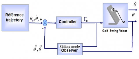
The controller-based sliding mode observer, which is given by Eq. (47), was tested by numerical simulation using the golf swing robot manipulator described in Section 2 as can be seen in Figure 3. The observer estimates the angular velocities of the robot using the joint angular positions measurements taking into account parameter uncertainties and external disturbances.
In this work, the external disturbance is considered as the shock due to a strike of the ball at the impact time 0.93 s. This shock is simulated by two pulses; the former joint is set equal to 50 N. m and 5 N. m for the latter joint.
In this context, we consider also the uncertainties of the parameters around 50% of the club nominal inertia, because under realistic conditions, the golfer uses several clubs.
Figure 3. Computed torque control law based Sliding mode observer
The reference trajectories are given as optimal motion trajectories of the robot, which have been determined in our previous work [15-17]. The simulation results are shown in these figures:
From Figure 4, we can notice that both input controls respect the physical conditions of actuators given in Table 1. It can also be noticed that the appearance of shock (opposite torques) at the impact time (tm=0.93s) corresponding to strike of the ball.
Figure 4. Computed torque controller based sliding mode observer
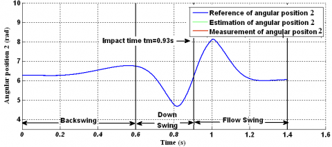
Figure 5. Angular position of joint 2
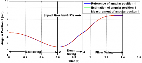
Figure 6. Angular position of joint 1
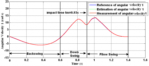
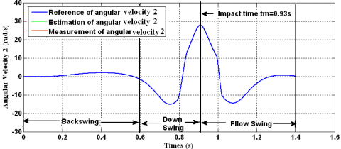
Figure 7. Angular velocity of joint 1
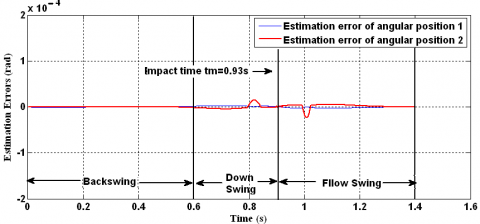
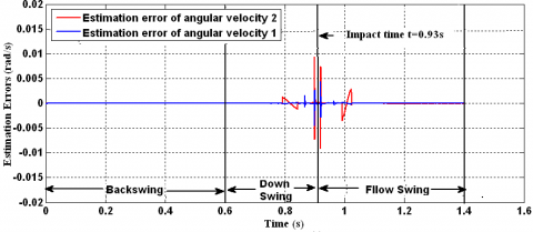
The evolution of estimated angular positions (see Figure 5 and Figure 6), and the estimated angular velocities (Figure 7 and Figure 8) follow the reference trajectories. Figure 9 and Figure 10 represent the estimation error of the positions and the velocities for both joints, respectively. These estimation errors are kept within a small variably rang and converge very quickly to zero in the backswing and follow through phases. However, in the downswing period, which represents the hyper dynamic motion, we can observe a slightly larger error around the impact time. This error is due to the non-linear structure of the joins stop. Because the sign switching function is applied in the observer structure, and the obtained error values always oscillate in a very small rang around zero, even after state estimations have already converged to the real states.
Through these simulation results, we can conclude that the proposed control-based observer provides a good closed-loop performance of the robot arm and ensure the estimation error convergence.
Figure 8. Angular velocity of joint 2
Figure 9. Estimation error of angular positions
Figure 10. Estimation error of angular velocities
In this paper, a robust Sliding Mode observer for a class of a hyper dynamic manipulation which is characterized by its nonlinear dynamics is proposed. As a case study, two-link golf swing robot is considered in our application.
This observer has been combined with a state feedback controller (computed torque) taking into account parametric uncertainties and external disturbances.
Numerical simulations tests show the effectiveness and robustness of the proposed approach, that the robot follows its optimal motion trajectories. After this work, we will focus on verifying these results through experiments. It is expected that the effects of the twisting motion of the wrist joint element and the shaft torsional vibrations will be improved.
In future work, we plan to adapt this proposed strategy for autonomous vehicles localization such as unmanned aerial vehicle and autonomous underwater vehicle.
|
${{\theta }_{i}}$ |
Generalized coordinates of joints i. |
|
$\theta _{i}^{\min },\theta _{i}^{\max }$ |
Free rotation range of joint i (minimum and maximum of ${{\theta }_{i}}$). |
|
$\theta _{2}^{lb}$ |
Maximum of rotation range of the joint stop in a clockwise direction. |
|
$\theta _{2}^{ub}$ |
Maximum of rotation range of the joint stop in an anticlockwise direction. |
|
$\tau _{i}^{\max },\tau _{i}^{\min }$ |
Maximum and the minimum active torque of joint i. |
|
${{t}_{0}}$ , ${{t}_{f}}$ |
Time of initial and final position. |
|
${{\Gamma }_{1,2}}$ |
Driving torque vector. |
|
${{\tau }_{i}}$ |
Active torque of joint i. |
|
${{\theta }_{i}},{{\dot{\theta }}_{i}},{{\ddot{\theta }}_{i}}$ |
Angle, angular velocity and acceleration of joint i.
|
|
$M(\theta )$ |
Inertia matrix. |
|
$\dot{\tilde{\theta}}$ |
Centrifuge and Coriolis matrix. |
|
$G(\theta )$ |
Gravity vector. |
|
${{k}_{w}}$ |
Stiffness scalar. |
|
${{c}_{w}}$ |
Damping scalar. |
|
$\tau _{2passif}^{_{\min }}$ |
Minimum passive torque of joint 2. |
|
$\tau _{2passif}^{_{\max }}$ |
Maximum passive torque of joint 2. |
|
${{\hat{x}}_{i}}$ |
Estimated state of ${{x}_{i}}$. |
|
${{\bar{x}}_{1}}$ |
State estimation errors. |
|
${{\Lambda }_{1}}$,${{\Lambda }_{2}}$ |
Positive definite constant diagonal matrices. |
|
${{\lambda }_{1}}$,${{\lambda }_{2}}$ |
Positive constants. |
|
${{\ddot{\theta }}_{r}},{{\dot{\theta }}_{r}},{{\theta }_{r}}$ |
Angular reference acceleration, angular reference velocity and angular reference position trajectories. |
|
${{k}_{p}}$ |
Diagonal positive definite matrices for proportional gain. |
|
${{k}_{v}}$ |
Diagonal positive definite matrices for derivative gain. |
|
$\dot{\tilde{\theta}}$ |
Angular velocity tracking error. |
|
$\tilde{\theta}$ |
Angular position tracking error. |
[1] Li, Z.W. (2017). Study on dynamic analysis and wearable sensor system for golf swing. Kochi University of Technology Doctoral Program Engineering Course. Thesis of Doctorat.
[2] Li, Z.W., Yoshio, I., Shunta, K., Kyoko, S. (2014). The effect of swing pattern on the release point and the club head speed. 3th International Conference on Multibody System Dynamics, Korea.
[3] MacKenzie, S.J. (2012). Club position relative to the golfer’s swing plane meaningfully affects swing dynamics. Sports Bio-mechanic, 2(11): 149-164. https://doi.org/10.1080/14763141.2011.638388
[4] Coleman, S., Anderson, D. (2007). An examination of the planar nature of golf club motion in the swings of experienced players. Journal of Sports Sci, 7(25): 739-748. https://doi.org/10.1080/02640410601113239
[5] Xu, C., Yang, Z.Z., Ming, A.G., Shimojo, M. (2012). Motion planning of golf swing robot. Elsevier Revue of Mechatronics. 22(1): 13-23. http://dx.doi.org/10.1016/j.mechatronics.2011.10.006
[6] Suziki, S., Inooka, H. (1999). A new golf swing robot model emulating golfer’s skill. Sports Engineering, 2(1): 13-22. http://dx.doi.org/10.1046/j.1460-2687.1999.00013.x
[7] Ming, A., Mita, T., Dhlamini, S., Kajitani, M. (2001). Motion control skill in human hyper dynamic manipulation an investigation on the golf swing by simulation. In Proceedings of the IEEE International Symposium on Computational Intelligence in Robotics and Automation, pp. 47-52. http://dx.doi.org/10.1109/CIRA.2001.1013171
[8] Ming, A., Kajitani, M. (2000). Human dynamic skill in high speed actions and its realization by robot. Journal of Robotics and Mechatronics, 12(3): 318-334. http://dx.doi.org/10.20965/jrm.2000.p0318
[9] Aicardi, M. (2007). A triple pendulum robotic model and a set of simple parametric functions for the analysis of the golf swing. International Journal of Sports Science and Engineering, 1(2): 75-86.
[10] Hoshino, Y., Kobayashi, Y., Yamada, G. (2005). Vibration control using a state observer that considers disturbances of a golf swing robot. International Journal JSME, 48(1): 60-69. http://dx.doi.org/10.1299/jsmec.48.60
[11] Hunt, E.A., Wiens, G.J. (2003). Design and analysis of a parallel mechanism for the golf industry. Proceedings of International Congress on Sound and Vibration, Stockholm, Sweden, pp. 7-10.
[12] Xu, C., Ming, A., Mak, K., Shimojo, M. (2007). Design for high dynamic performance robot based on dynamically coupled driving and joint stop. International Journal of Robotics and Automation, 22(4): 281-293. http://dx.doi.org/10.2316/Journal.206.2007.4.206-2999.
[13] Ming, A., Xu, C. (2012). Biologically Inspired Robotics. Taylor Francis Group, London, 55-84.
[14] Xu, C., Ming, A., Maruyama, T., Shimojo, M. (2007). Motion generation for hyper dynamic manipulation. International Journal of Mechatronics, Elsevier, 17(8): 405-416. http://dx.doi.org/10.1016/j.mechatronics.2007.05.002
[15] Aboura, S., Omari, A., Zemalache Meguenni, K. (2012). Optimizing motion planning for hyper dynamic manipulator. Journal of Electrical Engineering, 63(1): 21-27. http://dx.doi.org/10.2478/v10187-012-0003-0
[16] Aboura, S., Omari, A., Zemalache Meguenni, K. (2014). Motion planning and control of hyper dynamic robot. International Review of Automatic Control (IREACO), 7(1).
[17] Omari, A., Aboura, S. (2012). Comparative study on optimal motion planning based genetic algorithm for hyper dynamic robot arm. Mediterranean Journal of Measurement and Control, 8(3).
[18] Xu, C., Ming A., Shimojo, M. (2009). Motion planning for a golf swing robot based on reverse time symmetry and PGCTC control. In Proceeding of IEEE International Conference on Robotic and Automation ICRA’09. USA, 69-74. http://dx.doi.org/10.1109/ROBOT.2009.5152187
[19] Xu, C., Yang, Z., Ming, A., Shimojo, M. (2012). Motion planning of golf swing robot. Elsevier Review, 22(1): 13-23. http://dx.doi.org/10.1016/j.mechatronics.2011.10.006
[20] Aboura, S. (2016). Génération de mouvement optimal et commande d’un bras manipulateur hyper dynamique. Ph.D. Department of Automation. University of Sciences and Technology MB, Algéria.
[21] Aboura, S., Omari, A., Zemalache Meguenni, K. (2011). Observer based computed torque for hyper dynamic manipulator. International Conference on Automatic and Mechatronic CIAM 2011, University USTO-MB, Oran, Algeria.
[22] Venkatesan, M., Ravi, V.R. (2014). Sliding mode observer based sliding mode controller for interacting nonlinear system. Second International Conference on Current Trends, In Engineering and Technology- ICCTET'14, Coimbatore, India. http://dx.doi.org/10.1109/ICCTET.2014.6966254
[23] Utkin, V., Guldner, J., Shi, J.X. (2009). Slinding Mode Control in Eletro-Mechanical Systems. 2nd Eds., Publisher: Boca Raton, CRC Press, Taylor & Francis, London. https://doi.org/10.1201/9781420065619
[24] Vaidyanathan, S., Lien, C.H. (2017). Applications of sliding mode control in science engineering. Stadies in Computational Intelligence 709, Eds., Springer International Publishing. https://doi.org/10.1007/978-3-319-55598-0-14