Chungang Qu| Huiling Cao* | Shuang Sun | Meijian Xu
OPEN ACCESS
The fuel flow is a key indicator of the performance of aircraft engine. It helps to identify the performance degradation and failure of the engine. This calls for an aircraft engine model that can predict the fuel flow accurately throughout the flight, especially the climb phase. This paper performs stepwise linear regression of the data collected by a quick access recorder (QAR), and creates a model of the fuel flow of Boeing 737-700 in the climb phase. Firstly, the possible influencing factors of fuel flow were screened based on scatterplots and Pearson correlation coefficients (PCCs). Next, the selected factors were further modified and screened through similarity correction and power correction. On this basis, the fuel flow model for the climb phase was established through stepwise linear regression and corrected in the light of the tolerance and variance inflation factor (VIF) of each variable. The prediction results of the final model were basically in line with the actual QAR data.
fuel flow, quick access recorder (QAR), multiple linear regression, prediction
Aircraft engines are very important for flight safety [1]. Today’s complex and advanced technology systems require advanced and expensive maintenance strategies [2]. Because of the high cost of maintenance, gas turbine engines must be operated within specified physical limits [3]. Today’s aircraft engines are made safer by increasing the number of control parameters and sensors [4]. The engines have a complex mechanical system. Because aircraft engines operate at high temperatures, high pressures, and high speeds, there are lots of possibilities of various faults in the aircrafts [5].
Joly et al. searched the deterioration of the aircraft engines performance by using ANN [6]. Babbar et al. [7] used the prognostic methods for monitoring the aircraft engine performance. They estimated the performance of future flights by comparing the EGT values of two engines. Yukimoto and Syrmos [8] estimated the EGT value by using Support Vector Machine Expert Method and genetic algorithm methods. Anastassios [9] investigated the monitoring and diagnostic methods about gas turbine engines. Ackert [10] investigated about maintenance management in turbofan engines and relationship between engine deterioration and EGT margin value.
The fuel flow directly affects the power of aircraft engine, serving as a key indicator of engine performance. Considering its bearing on aircraft safety and economy, many airlines have attached great importance to the fuel flow [11]. Sun [12] developed a fault diagnosis algorithm for fuel flow sensor of aircraft engine. Cao [13] conducted a comprehensive correlation analysis (CCA) on the influencing factors of aircraft fuel consumption. Chati and Balakrishnan, [14-15] explored fuel flow modelling of aircraft engine through Gaussian process regression, and established a statistical model of the fuel flow of aircraft engine.
Airlines have taken various measures to improve fuel efficiency and reduce fuel cost. Fuel consumption is an important aspect of aircraft condition monitoring, for any abnormal change in fuel is directly related to aircraft failure. Focusing on CFM56-7B engine, Yılmaz [16] identified the relationship between exhaust gas temperature (EGT) and operating parameters. Mercer et al. [17] mentioned the monitoring and management of aircraft engine in the book Fundamental Technology Development for Gas-Turbine Engine Health Management.
The climb phase faces the most complex situation in the entire flight, with great changes in the outside air. In this phase, the aircraft is highly likely to fail and cause aviation accidents. Therefore, it is necessary to create a model of the fuel flow in the climb phase and use the model to monitor the fuel flow, aiming to detect abnormal changes in fuel flow in a timely manner. In this way, the fuel consumption will be monitored more efficiently, laying the basis for flight safety.
Drawing on theories on aircraft engine, fuel control and mathematical correlation, this paper carries out stepwise linear regression of the data collected by a quick access recorder (QAR), and creates a model of the fuel flow of Boeing 737-700 in the climb phase. The established model was verified with multiple sets of QAR data.
The QAR is an important data source for the monitoring of flight quality and engine state of the aircraft. The QAR data reflect the relationship between parameters, and imply the control law [18].
Due to their sheer volume and complex structure, the QAR data are difficult to be processed satisfactorily by traditional data analysis methods or modelling theories. For example, the Matlab-based numerical methods proposed by Mathews [19] cannot output intuitive or specific results, because the Matlab requires the user to master programming language and relevant professional knowledge.
To solve the problem, Carver [20] suggested doing data analysis using the Statistical Package for the Social Sciences (SPSS). The SPSS boasts numerous data interfaces and advanced methods for statistical analysis, offering a convenient way to process the QAR data and create relevant models. It is one of the most popular tools for statistical analysis.
The QAR data contain extremely rich information, including numerical parameters and character-type parameters. These parameters carry the information on all aspects of the flight. Each of them covers a specific field and has a unique importance.
For a flight, the first few parameters in the QAR data specify the number, time and origin/destination. The flight time is accurate to the second, and the origin/destination is marked according to the Annex of International Civil Aviation Organization (ICAO). After the initial parameters, there are a huge number of numerical parameters and character-type parameters representing the engine state. The numerical parameters may include: engine pressure ratio (EPR), low-pressure rotor speed (N1), thrust rod angle (TRA), flight altitude (ALT), pitch attitude angle (PITCH ATITUDE), etc.
According to the theories on engine fuel and control theory, the fuel consumption during the flight is affected by multiple factors. Hence, the fuel consumption modelling is essentially a multivariate statistical analysis. There are various methods for multivariate statistical analysis. The multiple linear regression stands out for its maturity and wide application. Therefore, this paper selects stepwise linear regression, a typical method of multiple linear regression, to analyze the statistics on the fuel flow of the aircraft in the climb phase.
3.1 Multiple linear regression model
In the multiple linear regression model, the population regression function (PRF) can be generally described as:
$\mathrm{Y}=\beta_{0}+\beta_{1} X_{1}+\beta_{2} X_{2}+\ldots+\beta_{p} X_{p}+\varepsilon$ (1)
where, ε is the random error; $\beta_{1}, \beta_{2}, \ldots, \beta_{p}$ are population regression coefficient. $\beta_{j}$ is also known as the partial regression coefficient, because it measures the mean variation of the dependent variable Y caused by the change of each unit of the independent variable Xj.
The above formula assumes that the regression relationship between the dependent variable Y and the independent variables X1, X2, X3,…, Xp is approximately a linear function. In the formula, the population regression coefficients are unknown and must be estimated based on the observed values of relevant samples.
Suppose there are n observed values, and $\beta_{1}, \beta_{2}, \ldots, \beta_{p}$ are the estimates of population regression coefficients. Then, the sample regression function of the multiple linear regression model can be described as:
$\hat{Y}=\hat{\beta}_{0}+\hat{\beta}_{1} X_{1}+\hat{\beta}_{2} X_{2}+\ldots+\hat{\beta}_{p} X_{p}+e,(\mathrm{p}=1,2, \ldots, \mathrm{n})$ (2)
where, e is the deviation between Y and its estimate $\hat{Y}$, i.e. the residual. Like the unary linear regression, multiple linear regression also requires several hypotheses.
3.2 Prerequisites and conditional tests for multiple linear regression
Linear regression is only suitable for modelling linearly correlated variables. Thus, the correlation between variables should be analyzed before linear regression. Correlation analysis is an exploratory method for statistical analysis. The results and purpose of correlation analysis provide guidance for further analysis.
Correlation analysis is mainly performed by graphical method and the calculation of correlation coefficient. The graphical method finds the pattern of the correlation between variables by drawing the relevant scatterplots. This exploratory approach should be combined with relevant correlation coefficients. As its name suggests, the calculation of correlation coefficient refers to computing the correlation coefficient by the method that suits the specific type of data.
3.2.1 Scatterplot
The scatterplot provides a visual representation of the relationship between two variables. To draw the scatterplot, a variable is taken as the horizontal axis and the other as the vertical axis. Then, the corresponding values of the two variables are marked one by one as the coordinate points in the Cartesian coordinate system. The shape, pattern and density of the point distribution reflect the correlation between the two variables.
3.2.2 Pearson correlation coefficient (PCC)
Unlike the traditional measure of covariance, the correlation coefficient is nondimensional. It measures whether two variables are linearly correlated. If so, the correlation coefficient can describe the direction and degree of the linear correlation between the two variables. The correlation coefficient was first proposed by Pearson, and thus called the Pearson correlation coefficient (PCC). The PCC is defined as follows:
$\rho=\frac{1}{n-1} \sum_{i=1}^{n}\left(\frac{y_{i}-\bar{y}}{s_{y}}\right)\left(\frac{x_{i}-\bar{x}}{s_{x}}\right)=\frac{\operatorname{Cov}(X, Y)}{s_{y} s_{x}}$ (3)
where, $\bar{x}$ and $\bar{y}$ are the mean values of the two samples; $s_{x}$ and $s_{y}$ are the standard deviations of the two samples; $\operatorname{cov}(Y, X)$ is the covariance of the samples. These parameters can be respectively calculated by:
$\bar{y}=\sum_{i=1}^{n} y_{i} / n$ (4)
$\bar{x}=\sum_{i=1}^{n} x_{i} / n$ (5)
$s_{x}=\sqrt{\sum_{i=1}^{n}\left(x_{i}-\bar{x}\right)^{2} /(n-1)}$ (6)
$s_{y}=\sqrt{\sum_{i=1}^{n}\left(y_{i}-\bar{y}\right)^{2} /(n-1)}$ (7)
$\operatorname{Cov}(X, Y)=\sum_{i=1}^{n}\left(x_{i}-\bar{x}\right)\left(y_{i}-\bar{y}\right) /(n-1)$ (8)
The PCC value falls between -1 and +1. If $|\rho| \approx 0$, then the two variables are not linearly correlated; if $|\rho| \approx 1$, then the two variables are completely linearly correlated. The direction of the linear correlation is specified by the sign of the PCC: “+” means positive correlation and “-” means negative correlation.
3.3 Stepwise linear regression
The stepwise linear regression is a multiple linear regression good at screening independent variables. By this method, the variables are both selected through forward propagation and deleted through backpropagation. During the bidirectional screening, any external variable can reenter the model, if it provides explicit explanations, and any internal variable will be removed, if it fails to pass the t-test.
In actual research, the linear correlation between dependent variable and the independent variable should be verified based on the scatterplot and the PCC, according to $\sum_{i=1}^{n}\left(y_{i}-\bar{y}\right)^{2}=\sum_{i=1}^{n}\left(\hat{y}_{i}-\bar{y}\right)^{2}+\sum_{i=1}^{n}\left(y_{i}-\hat{y}\right)^{2}$. Even if the linear correlation is confirmed, the multiple linear regression formula should be subjected to significance tests like F-test, t-test and R2-test, as well as the collinearity diagnosis.
The QAR-based fuel flow model was established in the light of theories on aircraft engine, fuel control and multiple linear regression. The flight consists of many phases, namely, taxi, takeoff, climb, cruise, descend, final approach and landing. Compared with the other phases, the climb phase sees great changes in fuel oil consumption and carries the typical features of the flight. Therefore, this section aims to establish a fuel flow model for the aircraft in the climb phase, that is, to determine the relationship between the fuel flow in the left engine and its influencing factors. For this purpose, a single set of QAR data was processed and analyzed on the SPSS, and then the fuel flow of the aircraft was constructed.
4.1 Parameter selection
The QAR data contains many parameters that may affect the fuel consumption in the climb phase, including Mach number (Mach), flight altitude (ALT), temperature, atmospheric environment, as well as engine parameters like low-pressure rotor speed (N1), high-pressure rotor speed (N2) and the thrust rod angle (TRA). Referring to the Aircraft Performance Manual, twelve parameters were selected preliminarily as the influencing factors of fuel consumption in the climb phase:
Flight altitude (ALT), Mach number (Mach), calibrated airspeed (CAS), engine pressure ratio (EPR), total temperature through the high-pressure compressor inlet (T2), low-pressure rotor speed (N1), high-pressure rotor speed (N2), thrust rod angle (TRA), total pressure at station 2 (P2), total air temperature (TAT), total pressure (TP), total temperature through the high-pressure compressor outlet (T3).
4.2 Similarity correction and power correction
Inspired by the theory of similarity for aircraft engines, the exhaust gas temperature (EGT), low-pressure rotor speed (N1), high-pressure rotor speed (N2) and fuel flow (FF) were corrected under the same atmospheric conditions, eliminating the influence of external conditions on engine performance parameters. The corrections also make the data of different flights comparable. The engine performance parameters can be corrected by:
$N_{1 c o r}=N_{1 r a v} / \sqrt{T_{2} / T_{0}}$ (9)
$N_{2 c o r}=N_{2 r a v} / \sqrt{T_{2} / T_{0}}$ (10)
$E G T_{c o r}=E G T_{r a v} /\left(T_{2} / T_{0}\right)$ (11)
$F F_{c o r}=F F_{r a w} /\left(\left(T_{2} / T_{0}\right)^{x}\left(P_{2} / P_{0}\right)\right)$ (12)
where, the suffix “raw” stands for raw data; the suffix “cor” stands for corrected data.
Besides the different external conditions, the thrust during the flight also affects the parameters of engine performance. For Pratt & Whitney’s engines, the thrust value is usually characterized by the EPR.
In the cruise state, the engine thrust differs from flight to flight. Therefore, the performance parameters of the same engine in different flights may not be comparable, even if they have undergone similarity corrections. To solve the problem, the data were subjected to power correction based on the engine baseline, and converted into parameters under the same EPR.
In its Electronic Control Module (ECM) Repair Guide, Pratt & Whitney defined engine baseline as the relationships between performance parameters (N1, N2, EGT and FF) and EPR after similarity corrections. The relationships are approximately linear (Figure 1).
Figure 1. Relationships between performance parameters and the EPR
According to the above relationships, the performance parameters can be corrected under the same preset thrust, knowing the slopes (kN1, kN2, kEGT and kFF) of the relationship curves in Figure 1. The power correction formula can be expressed as:
$D A T A_{c o r}=D A T A_{r a w}-k \cdot\left(E P R_{r a w}-E P R_{s t d}\right)$ (13)
where, DATAraw are raw data; DATAcor are corrected data; EPRraw is actual thrust; EPRstd is the preset standard thrust; k is the slope of the relationship curve between each parameter and EPR.
4.3 Fuel flow model for the climb phase
4.3.1 Preliminary model
Since there are many independent variables, the PCC was calculated to verify the linear correlation between each independent variable and the dependent variable (fuel flow), and judge the degree of influence of each independent variable that is linearly correlated with fuel flow. The PCC of each independent variable is listed in Table 1 below.
Table 1. The PCC of each independent variable
|
|
ALT |
MACH |
CAS |
EPR |
T2 |
N1 |
N2 |
TRA |
P2 |
TAT |
TP |
T3 |
|
PCC |
-0.996 |
-0.977 |
0.255 |
-0.935 |
-0.988 |
-0.920 |
0.929 |
0.730 |
0.991 |
0.989 |
0.991 |
0.937 |
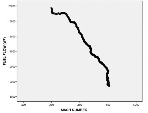
Figure 2. The scatterplot between Mach and FF
However, the PCC alone cannot fully demonstrate the existence or degree of the linear correlations. Hence, the scatterplot between each independent variable and the dependent variable was drawn to further judge the nonlinear relationship. The scatterplot between Mach and FF is presented in Figure 2 as an example.
As shown in Table 1, the PCCs of independent variables like ALT, Mach and N2 were close to one, indicating that these variables have great impacts on the fuel flow in the climb phase. By contrast, the CAS had the smallest absolute value of the PCC (0.255). This means the impacts of the CAS on the fuel flow is negligible. Thus, the CAS was excluded from our model.
4.3.2 Analysis of the preliminary model
The tolerance and variance inflation factor (VIF) of each variable in the preliminary linear regression model are shown in Table 2. The results show that the VIFs of all independent variables were greater than 10 (i.e. the tolerances were smaller than 0.1). Thus, the independent variables may have serious collinearity. Then, the eight variables in the preliminary model were rescreened and regressed again.
Table 2. The tolerance and VIF of each variable
|
|
ALT |
MACH |
EPR |
N1 |
N2 |
TRA |
TP |
T3 |
|
tolerance |
0 |
0.002 |
0.005 |
0.002 |
0.003 |
0.033 |
0.001 |
0.032 |
|
VIF |
3515.165 |
406.992 |
186.942 |
452.504 |
323.353 |
30.684 |
898.789 |
30.994 |
4.3.3 Correction of the preliminary model
Through the above analysis, ALT, EPR, TP, T3 and N1 were removed from our model, leaving only three independent variables: TRA, Mach and N2. Next, the fuel flow in the climb phase was modelled again through stepwise linear regression:
Y = -52734.966 + 760.761*N2L – 18025.937*MACH + 153.903*TRAL
4.3.4 General model
The above model was established through stepwise linear regression of only one set of QAR data. In real world scenarios, analysis results tend to have strong contingency if there are only a few data. To eliminate the contingency, this paper acquires 10 sets of QAR data from 12 flights of the same aircraft, and creates models through stepwise linear regressions on these data, using the SPSS. Excluding engine failure and abnormal external factors, seven fuel flow models were obtained for the climb phase, provided that the engine is working normally. The regression coefficients of the seven models were averaged to obtained a general fuel flow regression model:
$Y=-45438.275+683.682 * N_{2 L}-19542.839 * M A C H+145.254 * T R A_{L}$
4.4 Verification and prediction of the general model
The general model was tested by mean percentage error (MPE):
$(M P E)=1 / n \sum_{i=1}^{n}\left|\hat{Y}_{i}-Y_{i}\right|$ (14)
Statistics show that the MPE of the general model was 300.8347, revealling that the model accuracy falls in the acceptable range.
Furthermore, the general model was applied to predict the fuel flow of the aircraft in one of the remaining two flights. The prediction results were compared with the actual QAR data (Figure 3). The comparison shows that the prediction results basically agree with the actual data.
Figure 3. Comparison between the prediction results and the actual QAR data
Through stepwise linear regression, this paper models the fuel flow of Boeing 737-700 in the climb phase, verifies the accuracy of the model, and applies the model to predict the fuel flow of the aircraft in an actual flight. The model accuracy and prediction error both fell in the acceptable range.
Of course, the model accuracy could be further improved, especially the relative high contingency of the prediction results. The high contingency is attributable to the limited number of QAR data files. This problem will be solved in future research.
This work was financially supported by Civil Aviation University of China research fund: ZXH2012P007.
[1] Volponi, A.J. (2014). Gas turbine engine health management: Past, present, and future trends. Journal of Engineering for Gas Turbines and Power, 136(5): 051201-1. http://doi.org/10.1115/1.4026126
[2] Kim, S.H., Cohen, M.A., Netessine, S. (2007). Performance contracting in after-sales service supply chains. Management Science, 53(12): 1843-1858. http://doi.org/10.1007/978-3-319-32441-8_4
[3] Yu, B., Liu, D.D., Zhang, T.H. (2011). Fault diagnosis for micro-gas turbine engine sensors via wavelet entropy. Sensors, 11(12): 9928-9941. http://doi.org/10.3390/s111009928
[4] Schadow, K., Horn, W., Pfoertner, H. (2010). Sensor and actuator needs for more intelligent gas turbine engines. ASME Turbo Expo 2010: Power for Land, Sea, and Air, 155-167. http://doi.org/10.1115/GT2010-22685
[5] Xu, H., Jiang, D., Liang, L. (2012). Application of fuzzy-rough set theory and improved SMO algorithm in aircraft engine vibration fault diagnosis. In Proceedings of the IEEE 2012 Prognostics and System Health Management Conference (PHM-2012 Beijing), pp. 1-6.
[6] Joly, R.B., Ogaji, S.O.T., Singh, R., Probert, S.D. (2004). Gas-turbine diagnostics using artificial neural-networks for a high bypass ratio military turbofan engine. Applied Energy, 78(4): 397-418. http://doi.org/10.1016/j.apenergy.2003.10.002
[7] Babbar, A., Syrmos, V.L., Ortiz, E.M., Arita, M.M. (2009). Advanced diagnostics and prognostics for engine health monitoring. Aerospace Conference, 2009 IEEE, 7-14. http://doi.org/10.1109/AERO.2009.4839657
[8] Yukitomo, A.R., Syrmos, V.L. (2010). Forecasting gas turbine exhaust gas temperatures using support vector machine experts and genetic algorithm. Control & Automation. IEEE, 345-350. http://doi.org/10.1109/MED.2010.5547692
[9] Anastassios, G. (2013). Engine condition monitoring and diagnostics. Intech, ISBN 978-953-51-1166-5. http://doi.org/10.5772/54409
[10] Ackert, S. (2015). Engine maintenance management, Managing technical aspects of leased assets. Madrid, Spain, 1-31.
[11] Cao, H.L., Jia, C. (2013). Research of fuel flow regression model of aircraft climb phase based on QAR. Journal of Civil Aviation University of China, 31(3): 31-35. http://doi.org/CNKI:SUN:ZGMH.0.2013-03-009
[12] Sun, Z.R., Sun, Y.G. (2014). Research of real-time fault diagnosis platform of aero-engine's fuel flow sensors. 2014 International Conference on Mechanical. Electronic and Engineering Technology, 538: 206-209. http://doi.org/10.4028/www.scientific.net/amm.538.206
[13] Cao, H.L., Wang, X.Y. (2016). Research on aircraft fuel consumption influencial parameters in climbing phase based on comprehensive relevance. Journal of Civil Aviation University of China, 34(2): 19-22. http://doi.org/CNKI:SUN:ZGMH.0.2016-02-005
[14] Chati, Y.S., Balakrishnan, H. (2017). A gaussian process regression approach to model aircraft engine fuel flow rate. 8th ACM/IEEE International Conference on Cyber-Physical Systems, pp. 131-140. http://doi.org/10.1145/3055004.3055025
[15] Chati, Y.S., Balakrishnan, H. (2016). Statistical modeling of aircraft engine fuel flow rate. 30th Congress of the International Council of the Aeronautical Sciences, Daejeon, Korea, 1-10.
[16] Yilmaz, I. (2009). Evaluation of the relationship between exhaust gas temperature and operational parameters in cfm56-7b engines. Proceedings of the Institution of Mechanical Engineers Part G Journal of Aerospace Engineering, 223(G4): 433-440. http://doi.org/10.1243/09544100JAERO474
[17] Mercer, C.R., Simon, D.L., Hunter, G.W., Arnold, S.M., Reveley, M.S., Anderson, L.M. (2007). Fundamental technology development for Gas-Turbine Engine health management. Aerospace 2007 Conference, CA, United States, NASA-20070022364.
[18] Liu, Y. (2011). Research on the control law of PW4077D engine bleed valve based on association rule mining. Public Communication of Science & Technology, 16: 238-239.
[19] Mathews, J.H. (2009). Numerical methods using MATLAB. Publishing House of Electronics Industry. http://doi.org/10.1007/978-1-4842-0154-1
[20] Carver, R.H. (2011). Doing data analysis with SPSS version 12.0.Thomson/Brooks/Cole.