Mohammad Vardi| Mehdi Neyestani | Ali Ghorbanian*
OPEN ACCESS
In today's competitive world, it is very important for organizations to select suppliers according to price, quality, satisfactory service and timely delivery. Since a considerable portion of production costs is associated with purchasing raw materials from suppliers, selection of the right suppliers and allocation of optimal order quantities plays an important role in the success of an organization. So far, extensive research has been conducted in the context of supplier selection, and multi-criteria decision-making techniques are the common approach used to select the appropriate option. Recently, some studies in the context of supplier selection considered variable assumptions like quantity discount possibility. So, the aim of this study is modeling the supplier selection problem based on incremental and wholesale discounts and comparing the results of them like best selected supplier(s) and optimal order allocation to them. And solve a big problem with GA and NSGA algorithms and comparing with each other’s for this an integrated three-stage approach has been proposed by combining fuzzy AHP and Extended Analysis Method for the supplier selection problem and develop a GA&NSGA algorithms. Finally, the performance of the proposed approach and proposed algorithms has been appraised by numerical examples.
supplier selection, fuzzy AHP method, discount, weighting method, GA and NSGA-II
Supply chain includes all the stage which are involved in satisfying customer's need directly & indirectly. Supply chain not only includes the suppliers, but also involves transportation, stores, retailers & customers, too. The manufacturing firms should decrease the extra costs of supply chain to retain their competitive position. For example, it should be better to outsource parts & services which are not strategic goods of manufacturer. When a firm decides outsourcing, its main challenge is supplier selection problem [1]. Selecting of suppliers is one of the main parts in supply chain as well as it has turned to a strategic decision in supply chain during recent years. In manufacturing industries, procurement of raw materials includes approximately 70 % of the manufacturing costs. In such a condition, firm's purchasing department plays an important role in cost decrement and supplier selection is an important task in purchasing management [2].
Supplier selection problem is two types:
(1) Supplier selection without capacity restrictions. i.e. It can satisfy all the buyer’s needs.
(2) Supplier selection with capacity restrictions. It means that, the supplier can’t satisfy all the buyer’s needs. So, buyer has to supply some of his requirements by another supplier [3].
In supplier selection problem, we are facing with a multi-dimensional problem. Thus, researchers use single or mixed multi-criteria decision-making techniques for supplier selection problem.
Amid et al. used a weighted multi-objective fuzzy model with three objectives including price and lead-time minimization and quality maximization for order allocating while each supplier offer various quantity discount [4, 5]. Have used goal programming approach & Fuzzy TOPSIS for supplier selection. The relationship closeness, quality, delivery ability, guarantee & expire date criteria have been used in their research. Network analysis process and mixed integer linear programming have been applied by Liao and Kao to investigate quantitative & qualitative criteria in supplier selection. They have determined the optimal order allocation to each supplier with the aim of maximizing purchase value, minimizing consuming budget & the least failure rate. 14 criteria have been investigated in 4 clusters; profit, opportunity, cost & risk [6]. Demirtas & Üstün applied a fuzzy approach for supplier selection in a washing machine company among three candidates [7]. A multi-criteria intuitionistic fuzzy group decision making has been exploited by Kilincci & Onal [8], 2011 to rank 5 supplier. Boran et al. [9] proposed an AHP-based approaches for supplier evaluation and they used quality, serving level, innovation & management and financial conditions as selection criteria. Bruno et al. [10] have presented a two-layer model for supplier selection. They proposed a multi-objective mixed integer programming model. Shahroodi & Hassani [11] suggested a mathematical model to select suppliers through using DEA integrated approach and wholesale ownership cost with a case study in construction value chain of Irankhodro industry. They have introduced the most efficient supplier with the least wholesale cost & have presented solutions for achieving to efficiency by the other part makers. Tabriz & Azar [12] have presented a fuzzy decision making process model for strategic supplier selection. The supplier selection & order allocation for the selected suppliers is very complicated when quantity discounts are considered in problem. We can find supplier selection problem & order allocating simultaneously in the researches of Yücel and Güneri [2], Sadrian and Yoon [13]. Recently some other studies like Perić and Babić [14], investigated supplier selection & order allocating problem through using Fuzzy AHP hybrid approach & multi-objective linear programming. Kannan et al. [15] have used a Fuzzy simulation based Fuzzy TOPSIS method for proper suppliers selection by evaluation of 4 criteria; operational strategy, service quality, innovation & risk. Zouggari and Benyoucef [16] have investigated the problem of dynamic supplier selection. Sivrikaya et al. [17] have investigated the problem of supplier selection in textile industry they have used two phases that consist of fuzzy AHP and goal programming. Ayhan and Kilic [18] have presented a two stage approach for supplier section problem, in the first stage, the relative weight of each criterion for each type of item are determined via F-AHP technique and in second stage these output are used as inputs in the MILP model to determine the supplier selection. In this research 4 criteria namely, price, quality, delivery time performance, and after sales performance are used for altenatives evaluation. Like the other research, they applied wholesale discount in their model. New approaches for supply chain coordination problem are developed by Arshinder & Deshmukh [21, 20] and Cardenas & Barron [22]. A multi-objective supplier selection and order allocation problem with fuzzy objective are studied by Kazemi et al. [23].
As it can be seen, former researches mostly consider wholesale discount in their studies and not only don't apply other type of discount, but also there isn't any research that compares the results of these two types of discount. So one of the main contribution of this study is investigating and modeling of incremental discount and also comparing the result of them toward wholesale discount.
The main differences of this study than previous research is:
(1) As much as the authors are aware, this study for the first time considers the incremental discount in the supplier selection problem.
(2) Unlike previous researches that just solve the model just for small size problem, in this work by dealing with large size problem, we have investigated the efficiency of exact solution according to time consuming.
(3) In previous studies, Weighted Method have been used to solve the Multi-Objective optimization problem, however we applied a non-dominated solution for solving the problem.
(4) In spite of previous studies, this is the first work that used meta-heuristic algorithms (e.g. NSGA II) to solve multi-objective optimization problems.
This research tries to investigate the supplier selection problem while there are some restrictions on supplier’s capacity, quality and so on as well as a supplier can’t satisfy all of the buyer’s demand lonely. So, in this research, a two-stage approach has been used for modeling & supplier selection Problem Solving as well as allocating order to them in quantitative discount existing condition for various levels. In the first stage, an integrated fuzzy AHP- approach & extent analysis have been used for determining criteria weight. In second stage, the multi-objective problem has changed to a single-objective problem through weight method as well as single-objective modeling & problem solving have been done in two incremental & wholesale discounts mode.
Research structure is as follow; in the second section, a brief description on the used methods by the research such as calculating fuzzy numbers (the reason for fuzzy numbers will be explained), introducing extent analysis method, introducing weight methods have been presented. Then in the third section, problem mathematical modeling in partial & wholesale discounts existing condition for order quantities has been presented. In forth section, model performance in two partial & wholesale discounts mode has been compared by a numerical example to investigate the accuracy of the presented model. Finally, in the fifth section, conclusion & recommendations for future studies have been presented.
In this section, before modeling & problem solving, a brief description on the used techniques in the research & their way of calculating has been presented. In this part, at first the way of calculating fuzzy numbers by some decision makers has been presented; then, the extent analysis method has been introduced; finally, a brief description has been presented on the weighed method which its weights are being calculated by extent analysis method. The way of calculating fuzzy numbers in group decision making mode In fact, in a group decision making a group of individual comment on a special issue. In such a condition, the way of determining final resulted conclusion from the done decisions by the decision makers is important. Thus, this section tries to represent the way of calculating resulted conclusion from group decision making. It should be point out that the done decisions by the decision makers are being represented lingual. Therefore, the pre-determined triangular fuzzy numbers have been used for each of lingual variables. The way of calculating the resulted fuzzy numbers from group decision making is follow; At first, each of the decision makers are being requested to fill out criteria comparison questionnaire (these decision makers can compare the criteria individually or by group & in interaction with each other). This research has considered that each of decision makers have compared the criteria independently. Equations (1), (2) & (3) are being used for achieving to a fuzzy number resulted from n decision makers while decision makers do compare the criteria independently [16].
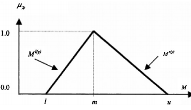
Figure (1) illustrates display of triangular fuzzy numbers. In this figure, the horizontal axis indicates triangular fuzzy numbers include three l, m & u values as well as the vertical axis indicates the related membership function to horizontal axis values and is calculated according to equation (4).
Figure 1. Triangular fuzzy numbers display
$l_{ij}={min}_k (l_{ijk})$ (1)
$m_{ij}={(\prod_{k=1}^n m_{ijk} )}^{(1/n)}$ (2)
$u_{ij}={max}_k (u_{ijk})$ (3)
In above equations, $l_{ij}$ , $m_{ij}$ & $u_{ij}$ are equivalent with the left value, average value & right value of resulted triangular fuzzy number through group decision making by k number for $i^{th}$ value of the $j^{th}$ supplier, respectively. K index represents the made decision by of $k^{th}$ decision maker.
$μ_M ̃ =\left\{\begin{array}{rl}0, x<l\\(x-l)/(m-l), l≤x≤m,\\(u-x)/(u-m),m≤x≤u,\\0, x≥u\end{array} \right.$ (4)
In relation (4), $μ_M ̃ $ indicates multi-value membership function by x values.
The fuzzy numbers are intuitively & easily useable to represent decision maker’s qualitative assessments.
Each fuzzy number can be indicated by its right & left values of membership degree as follow:
$M ̃=(M^{l(y)},M^{r(y)})=(l+(m-l)y, u+(m-u)y), yϵ[0,1]$ (5)
In AHP method, a cut of 1 to 9 discrete numerical scale is used for decision making on a criterion priority to other criteria while, fuzzy numbers or lingual values are being used in fuzzy AHP. When fuzzy numbers are being used in AHP technique, its way of solving will differ from the way of solving definite AHP. One of the most common methods for solving fuzzy AHP is extent analysis method which has been presented by Chang [17]. In this method, the “extent” is being valued by fuzzy numbers. The value of fuzzy compound degree can be achieved by the resulted fuzzy values from extent analysis for each criterion as follow;
In supplier selection problem, it is assumed that X={${x1,x2,…,xn}$} represents alternatives set as objective set as well as U={${u1,u2,…,um}$} represents set of supplier selection criteria as the goal set. According to extent analysis method, at first each of objective are chosen and the extent analysis is being done for each $g_i$ ideal, respectively. Therefore, m is the extent analysis value for each measurable objective which is represents as follow;
Where All $M_{g_i}^j$ are triangular fuzzy numbers. Generally, extent analysis method can be summarized in below steps;
First stage: Calculating fuzzy compound extent value according to the $i^{th}$ objective.
$s_i=\sum_{j=1}^m\quad m_{g_i}^j×{[\sum_{i=1}^n\quad\sum_{j=1}^m\quad M_{g_i}^j]}^{-1}$ (6)
The below equations represent the way of calculating ${[\sum_{i=1}^n\quad\sum_{j=1}^m\quad m_{g_i}^j]}^{-1}$ & $\sum_{j=1}^m\quad m_{g_i}^j$
$\sum_{j=1}^m\quad m_{g_i}^j=(\sum_{j=1}^m\quad l_j, \sum_{j=1}^m\quad m_j, \sum_{j=1}^m\quad u_j)$ (7)
${[\sum_{i=1}^n\quad\sum_{j=1}^m\quad m_{g_i}^j]}^{-1}=(\frac{1}{\sum_{i=1}^n\quad u_i}, \frac{1}{[\sum_{i=1}^n\quad m_i}, (\frac{1}{\sum_{i=1}^n\quad l_i})$ (8)
Second stage: Determining the possibility of $M_2=(l_2,m_2,u_2 )≥M_1=(l_1,m_1,u_1)$.
$V(M_2≥M_1)=\begin{cases}1, & \text{if}m_2≥m_1\\0, & \text{if}l_1≥u_2\\\frac{l_1-u_2}{(m_2-u_2)-(m_1-l_1)} , otherwise\end{cases}$ (9)
To compare, $M_1$ & $M_2$, the values of $V(M_1≥M_2)$ & $V(M_2≥M_1)$ should be calculated.
Third stage: Determining objective weight vector.
$\acute{W}=((\acute{d}(A_1), \acute{d}(A_2 ),…,\acute{d}(A_n ))^T, \\A_i (i=1,2,…,n), \acute{d}(A_i )=minV (s_i≥s_k ) \\k=1,2,…,n; k≠n$ (10)
Fourth stage: Determining normalized weight vector.
$W=((d(A_1 ),(d(A_2 ),…,(d(A_n))^T$ (11)
The weight method is one of the most applicable methods in modeling & solving multi-objective optimization problem in spite of being easy. In this method, a weight is considered for the problem various objective functions. This weight represents the importance & relative-priority of the objectives to each other. Since, the supplier selection problem & allocating order to them is of multi-objective optimization problems; thus, this research tries to use weight method for modeling & solving it. Notable point in weight method is the way of calculating the weights. So, the extent analysis method is used for determining relative weights of criteria to each other. After calculating relative weights of criteria to each other, the multi-objective linear programming modeling & solving it is done by the weight method. In the below part the way of changing the multi-objective problem to single-objective problem through using weight method has been represented.
$Max(Min) f_i (x), i=1,2,…,n\\S.t.\\g_i (x)≤or≥b_i, i=1,2,…,n\\x_i≥0.$ (12)
$Max(Min)w_1.f_1(x)+w_2.f_2(x)+…+w_n.f_n(x)\\S.t.\\g_i (x)≤or≥b_i, i=1,2,…,n\\x_i≥0$ (13)
This research tries to investigate supplier selection problem in two partial & wholesale discounts mode for order quantity. So, in this section two model have been presented for the possibility of existing partial & wholesale discount.
5.1 Mathematical model with the possibility of existing partial discount for order quantity
Supplier selection problem is a problem with multiple criteria. The considered criteria in this research are cost, quality & delivery time, respectively. These criteria are of the most important criteria which are used in the related researches to supplier selection as well as their application in various researches during recent years has been presented in table (1) in the appendixes. So, these three criteria have been used in this research as the main criteria in selecting proper supplier. Multi-objective integer linear programming modeling in the special partial discount condition for order quantity which has not been presented in the former researches has been presented in this section. Partial discount for order quantity is that the price is different for each determined quantity interval as well as wholesale price is being measured aggregately while in wholesale discount, all of the purchased quantities are being calculated by the related prices to the same price interval.
The model variables & parameters are being described before modeming the problem.
Variables;
$X_{ij}$ : Number of the purchased units from $i^{th}$ supplier in $j^{th}$ price level.
$Y_{ij}$: Zero & one variable for $i^{th}$ supplier $j^{th}$ price level.
Parameters;
$P_{ij}$: Product price for the $i^{th}$ supplier in the $j^{th}$ level.
$V_{ij}$: The length of the order interval from the $i^{th}$ supplier in the $j^{th}$ price level.
D: the demand of whole period.
$M_i$: The price levels of the $i^{th}$ supplier.
$C_i$: The capacity of the $i^{th}$ supplier.
$F_i$: The percentage of delayed items for the $i^{th}$ supplier.
$Q_i$: Quality of the $i^{th}$ supplier items.
n: Numbers of the suppliers.
$MinZ_1=\sum_{i=1}^n\quad p_ix_{i,1}+p_{i,2}\bullet(x_{i,2})+ +p_{i,m}\bullet(x_{i,m})$ (14)
$MaxZ_2=\sum_{i=1}^n\quad Q_i \sum_{j=1}^{mi}\quad x_{i,j}$ (15)
$MinZ_3=\sum_{i=1}^n\quad F_i\sum_{j=1}^{mi}\quad x_{i,j}$ (16)
S.t.
$\sum_{i=1}^n\quad\sum_{j=1}^{mi}\quad x_{i,j}≥D$ (17)
$\sum_{j=1}^{mi}\quad x_{i,j}≤ C_i i=1,2,...,n$ (18)
$V_{i,j}Y_(i,j)≤x_{i,j}, i=1,...,n, j=1,..., m$ (19)
$x_{i,j}≤v_{i,j}\bullet Y_{i,j-1} i=1,2,...,n, j=1,2,..., m_i$ (20)
$\sum_{j=1}^m\quad y_{ij}≤m, ∀iϵ i=1,…,n$ (21)
$Y_{i,j}=0 or 1 i=1,2,…,n, j=1,2,…$ (22)
$x_{i,j}≥0 , Integer i=1,2,…,n , j=1,2,…,m_i$ (23)
In the above model, the (14), (15) & (16) relations which represent objective functions are price minimizing, quality maximizing & lead time minimizing in delivery, respectively. The (17) & (18) relations are limitations for demand & capacity, respectively. The (19) & (20) relations also, are the related limitations to partial discount. Finally, the (21) & (22) relations represent the limitation of variables being zero & one as well as being positive.
5.2 Mathematical model with the possibility of existing wholesale discount for order quantity
In this part, a mathematical model is presented with the wholesale discount existence for order quantity. Since, in wholesale discount unlike partial discount all the purchased items are being purchased with the related price to the same interval; here, instead the parameter of $\acute{V}_{i,j}$ order quantity interval length the parameter of $\acute{V}_{i,j}$ order quantity upper limit is used. So, mathematical model of supplier selection problem & allocating optimum order to them in wholesale discount condition will be as follow;
New parameter;
$\acute{V}_{i,j}$: Upper limit of order interval from the $i_{th}$ supplier in the $j_{th}$ price level
$MinZ1=\sum_{i=1}^n p_{i,1} x_{i,1} +p_{i,2}∙(x_{i,2} )+⋯+p_{i,m}∙(x_{i,m} )$ (24)
$Max Z2 =\sum_{i=1}^n Q_i \sum_{j=1}^{mi} x_{i,j} $ (25)
$MinZ3=\sum_{i=1}^n F_i \sum_{j=1}^{mi} x_{i,j} $ (26)
S.t.
$\sum_{i=1}^n \sum_{j=1}^{mi} x_{i,j}≥D$ (27)
$\sum_{j=1}^{mi} x_{i,j}≤ C_i i=1,2,….,n$ (28)
$\acute{v}_{i,j} Y_{i,j}≤x_{i,j}, i=1,…,n, j=1,…,m$ (29)
$x_{i,j}≤\acute{v}_{i,j}∙Y_{i,j} i=1,2,…,n , j=1,2,…,m_i $ (30)
$\sum_{j=1}^m y_{ij} ≤1 , ∀iϵ i=1,…,n$ (31)
$Y_{i,j}=0 or 1 i=1,2,…,n , j=1,2,…$ (32)
$x_{i,j}≥0 i=1,2,…,n , j=1,2,…,m_i$ (33)
All limitations of the above model are the same as the former model except the (29) & (31) which are for wholesale discount.
5.3 Normalization
In multi-objective optimization problem, when we have different objective functions with different scales, normalization of objective functions, play an important role in ensuring the consistency of optimal solutions.
There are different approaches for normalization and one of the simplest (but appropriate) approaches is to optimize each of the objectives individually first, then divide each objective by those optimum values and finally sum up all normalized terms as one objective function
Initially, each objective function is optimized separately and the negative ideal solution (worst solution) and positive ideal solution (best solution) of them are found. Since the values of objective function vary in different scales equation 34 and 35 is used for normalize the objective functions.
For minimization objective function
$f_i^N=\frac{NIS_f-f}{NIS_f-PIS_f}$ (34)
For maximization objective function
$f_i^N=\frac{f-NIS_f}{PIS_f-NIS_f }$ (35)
where, $f_i^N$ is the normalized value of the ith objective function, NIS is negative ideal solution of objective function and PIS is best solution or positive ideal solution at the end model is changed to a single-objective function by summing up all weighted functions as shown in Eq. (36).
$MAX(f)=\sum_{i=1}^n w_i f_i^N$ (36)
In this part, the implementation stages of supplier selection problem as well as their step by step solving to investigate the presented model validity is presented though giving a numerical example. In this example, three decision makers (to do group decision making), three supplier wilt limited capacity & the presenter of partial & wholesale discount for order quantity have been considered. The considered criteria in this example are cost, quality & lead time. Table 2 indicates the complete related information to price, quality & delivery as well as productive capacity for the three suppliers. The implementation steps of the recommended model for our example are as follow Table 2.
Table 2. Problem information
|
productive capacity |
Percentage lead time in delivery |
quality |
Purchase interval |
cost |
|
|
16000 |
0.1 |
80 |
[0-4000] |
15 |
Supplier 1 |
|
[4001- 8000] |
14.5 |
||||
|
[8001-16000] |
14 |
||||
|
15000 |
0.15 |
70 |
[0-3000] |
17 |
Supplier 2 |
|
[3001- 10000] |
16.5 |
||||
|
[10001-15000] |
16 |
||||
|
17000 |
0.3
|
95 |
[0-5000] |
13 |
Supplier 3 |
|
[5001- 11000] |
12.5 |
||||
|
[11001-17000] |
12 |
In this section, at first a questionnaire is prepared for the experts. This questionnaire includes questions through which the ecision makers are requested to represent their viewpoints on the criteria. Table (3) indicates an example of the filled questionnaire by the decision makers.
Table 3. The pair-wise comparison by the experts
|
lead time in delivery |
Quality (Q) |
Cost (C) |
First decision maker |
|
Very very imporant |
Equal importance |
1 |
Cost (C) |
|
Very very imporant |
1 |
|
Quality(Q) |
|
1 |
|
|
lead time |
In the next section, after filling the questionnaire by the experts the lingual values are changed to corresponding fuzzy numbers with them according to table (2) in the appendix. Table (5) indicates related fuzzy numbers to resulted lingual values from decision makers’ viewpoints. In this table C, Q & F represent cost, quality & lead time, respectively as well as D1, D2 & D3 represent decision maker 1, 2 & 3, respectively.
Table 4. Lingual values & their corres
|
Importance |
values |
|
The same importance |
(1,1,1) |
|
more Important portion |
(2/3,1,3/2) |
|
More Important |
(3/2,2,5/2) |
|
More & more important |
(5/2,3,7/2) |
|
Completely Important |
(7/2,4,9/2) |
Table 5. Corresponding fuzzy numbers with each decision makers’ preferences
|
D1 |
D2 |
D3 |
|
|
C/Q |
(1,1,1) |
(5/2,3,7/2) |
(1,1,1) |
|
C/F |
(5/2,3,7/2) |
(1,1,1) |
(3/2,2,5/2) |
|
Q/F |
(5/2,3,7/2) |
(2/7,1/3,2/5) |
(3/2,2,5/2) |
In the next section, resulted values of decision makers are being replaced with a fuzzy number through using (1), (2) & (3) equations.
Table (6) indicates these values.
Table 6. Fuzzy values of resulted mean from three decision makers
|
Lij |
Mij |
Uij |
|
|
C/Q |
1 |
1.44 |
3.5 |
|
C/F |
1 |
1.96 |
3.5 |
|
Q/F |
0.28 |
1.26 |
3.5 |
Table (7) indicates resulted triangular numbers from paired comparisons.
Table 7. Paired comparisons values resulted from table (6)
|
C |
Q |
F |
|
|
C |
(1,1,1) |
(1,1.44,3.5) |
(1,1.96,3.5) |
|
Q |
(1/3.51/1.44.,1/1) |
(1,1,1) |
(0.28,1.26,3.5) |
|
F |
(1/3.5,1/1.96,1/1) |
(1/3.5,1/1.26,1/0.28) |
(1,1,1) |
$S_{cost}= (3, 4.4, 8)\bigotimes(\frac{1}{19.071}, \frac{1}{11.42}, \frac{1}{6.137})=(0.157, 0.385, 1.303)\\S_{quality}=(1.56, 2.954,5.5)\bigotimes(\frac{1}{19.071}, \frac{1}{11.42}, \frac{1}{6.137})=(0.82,0.258,0.896)\\S_{delivery}=(1.571, 4.068, 5.57)\bigotimes(\frac{1}{19.071}, \frac{1}{11.42}, \frac{1}{6.137})=(0.082,0.356,0.9078)\\V(S_{cost}≥S_{quality})=1, V(S_{quality}≥S_{cost})=0.854\\V(S_{cost}≥S_{delivery})=1, V(S_{delivery}≥S_{cost})=0.963\\V(S_{quality}≥S_{delivery})=0.893, V(S_{delivery}≥S_{quality})=1\\\acute{d}(cost)=min(1,1)=1\\\acute{d}(Quality)=min(0.893,854)=0.854\\\acute{d}(Delivery)=min(0.963,1)=0.963\\\acute{W}=(1,0.854,0.963)\\$
The normalized resulted weight is as follow:
WG= (0.36, 0.3, 0.34)
Second step: Changing multi-objective optimizing model to single-objective model.
In this section, after determining the weight significance of each objective functions, multi-objective linear programming model is changed to single-objective model. The single-objective model is as follow for the example of partial & wholesale discount mode;
So in this section, we intend to normalize objective functions according to above mentioned approach. For the first step, we solve the single objective optimization problem for each objective function, to obtain the optimum value of them. Table (8), show the optimum value of objective functions.
Table 8. PIS and NIS for z1 to z3
|
Function |
PIS |
NIS |
|
Z1(min is best) |
249000 |
313000 |
|
Z2(max is best) |
1855000 |
1450000 |
|
Z3(min is best) |
22 |
55.5 |
$MAX Z=0.36*((313000-(15x_11+14.5x_12+14x_13+17x_21+16.5x_22+16x_23+13x_31+12.5x_32+12x_33 )))/(313000-249000)+0.3*((80 (x_11+x_12+x_13 )+70 (x_21+x_22+x_23 )+95(x_31+x_32+x_33 ))-1450000)/(1855000-1450000)+0.34*(55.5-(0.001(x_11+x_12+x_13 )+0.0015(x_21+x_22+x_23 )+0.003(x_31+x_32+x_33 )))/(55.5-22)$
S.t.
$x_{11}+x_{12}+x_{13}+x_{21}+x_{22}+x_{23}+x_{31}+x_{32}+x_{33}=20000\\x_{11}+x_{12}+x_{13}≤16000\\x_{21}+x_{22}+x_{23}≤15000\\x_{31}+x_{32}+x_{33}≤17000\\4000*Y_{11}-x_{11}≤0\\x_{11}-4000≤0\\4000*y_{12}-x_{12}≤0\\x_{12}-4000*Y_{11}≤0\\8000*y_{13}-x_{13}≤0\\x_{13}-8000*Y_{12}≤0\\3000*y_{21}-x_{21}≤0\\x_{21}-3000≤0\\7000*y_{22}-x_{22}≤0\\x_{22}-7000*Y_{21}≤0\\ 5000*y_{23}-x_{23}≤0\\x_{23}-5000*Y_{22}≤\\5000*y_{31}-x_{31}≤0\\x_{31}-5000≤0\\6000*y_{32}-x_{32}≤0\\x_{32}-6000*Y_{31}≤0\\6000*y_{33}-x_{33}≤0\\x_{33}-6000*Y_{32}≤0\\Y_{11}+Y_{12}+Y_{13}≤3\\Y_{21}+Y_{22}+Y_{23}≤3\\Y_{31}+Y_{32}+Y_{32}≤3\\Y_{i,j}=0,1 , i=1,2,…,n j=1,2,….,m_i\\x_{ij}≥0, i=1,2,…,n , j=1,2,….,m_i, x_{ij}=INTEGER$
$x_{11}+x_{12}+x_{13}+x_{21}+x_{22}+x_{23}+x_{31}+x_{32}+x_{33}=20000\\x_{11}+x_{12}+x_{13}≤16000\\x_{21}+x_{22}+x_{23}≤15000\\x_{31}+x_{32}+x_{33}≤17000\\x_{11}-4000*Y_{11}≤0\\4001*Y_{12}-x_{12}≤0\\x_{12}-8000*Y_{12}≤0\\8001*y_{13}-x_{13}≤0\\x_{13}-16000*Y_{13}≤0\\x_{21}-3000*Y_{21}≤0\\3001y_{22}-x_{22}≤0\\x_{22}-10000*Y_{22}≤0\\10001*y_{23}-x_{23}≤0\\x_{23}-15000*Y_{23}≤\\x_{31}-5000*Y_{31}≤0\\5001y_{32}-x_{32}≤0\\x_{32}-11000*Y_{31}≤0\\11001*y_{33}-x_{33}≤0\\x_{33}-16000*Y_{32}≤0\\Y_{11}+Y_{12}+Y_{13}≤1\\Y_{21}+Y_{22}+Y_{23}≤1\\Y_{31}+Y_{32}+Y_{32}≤1\\Y_{i,j}=0,1 ,i=1,2,…,n j=1,2,….,m_i\\x_{ij}≥0,i=1,2,…,n ,j=1,2,….,m_i, x_{ij}=INTEGER$
Third step: Running the model & finding the optimum solution.
The optimum values have been achieved through running the two above mentioned model in GAMS software (Table 8);
As it can be seen in above Table, 1 & 3 supplies have been selected for demand supply in both partial & wholesale discount mode. But, way of order allocating is different in both modes. As it has been stated, in partial discount mode each order interval has its own special price as well as only the values of this interval will have this discount While in wholesale discount, all of the related order to the mentioned supplier are sold with the price of this order quantity in the same interval. Generally, the results indicate that both discounts have selected the same suppliers for order allocation as well as the order quantity for them is the same. The only difference in these two discounts is the way of calculating order wholesale price. This has been shown well in table (9) in the part of calculating the first objective function value (ZI). The cause of the second & third objective functions being the same in both kinds of the discounts is order quantity being the same for suppliers is both kinds of discount.
Table 9. Optimum values of objective functions & resulted variables from model solving
|
Variables |
Partial discount |
Normalized value |
Wholesale discount |
Normalized value |
|
Z1 |
257000 |
1 |
256002 |
0.89059375 |
|
Z2 |
1855000 |
1 |
1779985 |
0.814777778 |
|
Z3 |
54 |
0.045 |
43.998 |
0.343343284 |
|
X11 |
3000 |
|
0 |
|
|
X12 |
0 |
|
0 |
|
|
X13 |
0 |
|
8001 |
|
|
X21 |
0 |
|
0 |
|
|
X22 |
0 |
|
0 |
|
|
X23 |
0 |
|
0 |
|
|
X31 |
5000 |
|
0 |
|
|
X32 |
6000 |
|
0 |
|
|
X33 |
6000 |
|
11999 |
|
|
0.36*Z1+0.3*Z2+0.34*Z3 |
|
0.675 |
|
0.682 |
Srinivas and Deb [24] have instructed NSGA method for optimization multi objective problems. This algorithm use Darwin's principle of natural selection for to find the formula or optimal solution. But NSGA algorithm is highly sensitive to share fitness and other parameters. So for the second version of NSGA algorithm called NSGA-II was introduced in [25] by Deb et al. in the NSGA algorithm some of answer selected by using tournament selection from answer of each generation. note in this method the answer that there isn’t any answer better than it is best answer and has more point. Answers ranked and sorted based on how many answers there are better than them [26]. Fitness allocated to answer based on their ranks and not overcome of other answers. In the first, rank of answer and second, compaction distance are criteria for selecting in NSGA –II algorithm. The answer is more favorable that rank answer is less and has more compaction distance. The not overcome answer that obtained archived and sorted as elite.
Table 10. Parameters levels of algorithms
|
levels |
Symbols |
parameters |
algorithms |
|
0.4-0.6-0.8 |
Pc |
Crossover rate |
NSGAII |
|
0.1-0.3-0.5 |
Pm |
Mutation rate |
|
|
20-50-100 |
pop |
Pop size |
|
|
100-200-300 |
It |
iteration |
|
|
0.4-0.6-0.8 |
Pc |
Crossover rate |
GA |
|
0.1-0.3-0.5 |
Pm |
Mutation rate |
|
|
20-50-100 |
pop |
Pop size |
|
|
100-200-300 |
It |
iteration |
Table 11. Taguchi results to adjust parameter’s NSGA algorithm
|
Wholesale discount |
Practical discount |
It |
pop |
Pm |
Pc |
Number of experiments |
|
0.60199 |
0.624179 |
100 |
20 |
0.1 |
0.4 |
1 |
|
0.65644 |
0.635072 |
200 |
50 |
0.3 |
0.4 |
2 |
|
0.66566 |
0.667806 |
300 |
100 |
0.5 |
0.4 |
3 |
|
0.64461 |
0.642662 |
300 |
50 |
0.1 |
0.6 |
4 |
|
0.66679 |
0.644928 |
100 |
100 |
0.3 |
0.6 |
5 |
|
0.64456 |
0.620905 |
200 |
20 |
0.5 |
0.6 |
6 |
|
0.66269 |
0.663939 |
200 |
100 |
0.1 |
0.8 |
7 |
|
0.61330 |
0.645692 |
300 |
20 |
0.3 |
0.8 |
8 |
|
0.66295 |
0.61057 |
100 |
50 |
0.5 |
0.8 |
9 |
7.1 Adjusting parameter’s algorithms
In this study used Taguchi method to adjust the parameters of the proposed algorithms. In this way at the first different levels of parameters be determined. Related parameters and values of GA& NSGA II algorithms are given in Table 10.
It is available of the value of parameters after running using the signal to noise. This graph is available for GA&NSGA algorithms that is showed in Figures 2 and 3.
At the end of each replication, a final answer has calculated by using weights that are obtained from fuzzy AHP method. The GA and NSGA run for 10 times and averaged for value can be seen in table 11 the final answer of Pareto solution is shown in Z.
Table 12. Taguchi results to adjust parameter’s GA algorithm
|
Wholesale discount |
Practical discount |
It |
pop |
Pm |
Pc |
Number of experiment |
|
0.67001 |
0.65481 |
100 |
20 |
0.1 |
0.4 |
1 |
|
0.67522 |
0.67045 |
200 |
50 |
0.3 |
0.4 |
2 |
|
0.67599 |
0.67332 |
300 |
100 |
0.5 |
0.4 |
3 |
|
0.66974 |
0.67007 |
300 |
50 |
0.1 |
0.6 |
4 |
|
0.67318 |
0.66916 |
100 |
100 |
0.3 |
0.6 |
5 |
|
0.67621 |
0.66679 |
200 |
20 |
0.5 |
0.6 |
6 |
|
0.67036 |
0.66691 |
200 |
100 |
0.1 |
0.8 |
7 |
|
0.67531 |
0.66982 |
300 |
20 |
0.3 |
0.8 |
8 |
|
0.67525 |
0.66855 |
100 |
50 |
0.5 |
0.8 |
9 |
Figure 2. Signal to noise for GA algorithm
Figure 3. Signal to noise for NSGA algorithm
Table 13. Best value for parameters of GA and NSGA algorithms
|
Value of parameter (wholesale discount) |
Value of parameter (practical discount) |
Symbol |
parameters |
algorithms |
|
0.6 |
0.4 |
Pc |
Crossover rate |
NSGAII |
|
0.5 |
0.1 |
Pm |
Mutation rate |
|
|
100 |
100 |
pop |
Pop size |
|
|
200 |
300 |
It |
iteration |
|
|
0.4 |
0.6 |
Pc |
Crossover rate |
GA |
|
0.5 |
0.3 |
Pm |
Mutation rate |
|
|
20 |
100 |
pop |
Pop size |
|
|
200 |
300 |
It |
iteration |
Table 14. Value of GA and NSGA
|
NSGA for practical |
GA for practical |
GA for wholesale |
NSGA for wholesale |
|
|
3586 |
3555 |
8838 |
8093 |
X1 |
|
60 |
93 |
100 |
5 |
X2 |
|
16355 |
16361 |
11067 |
11904 |
X3 |
|
259070 |
259238 |
258236 |
256235 |
Z1 |
|
1844805 |
1845205 |
1765405 |
1778670 |
Z2 |
|
52.7400 |
52.7775 |
42.189 |
43.812 |
Z3 |
|
20000 |
20000 |
20000 |
20000 |
X1+ X2+ X3 |
|
0.668 |
0.667 |
0.677 |
0.681 |
Normalized SAW |
Table 15. GA and NSGA error parentage
|
GA Error Parentage |
NSGA Error Parentage |
Value of GA |
Value of NSGAII |
Optimal Normalized value |
|
|
1.18 |
1.03 |
0.667 |
0.668 |
0.675 |
Practical discount |
|
0.73 |
1.02 |
0.677 |
0.681 |
0.682 |
Wholesale discount |
Appropriate values for the parameters of algorithm NSGAII and GA have been reported in Table 13.
Then the given example has solved by using the optimal value is obtained that has shown in table 14. Compared the obtained value with the optimal value is known as a very low percentage of errors, especially in the NSGA algorithm that this reflects the accurate of algorithms are used. Table 15 Shows value of errors.
Now given that accuracy of algorithms is evaluated then a big size problem has solved in both wholesale and practical discount. This problem can be seen in appendix 2. In this problem number of supplier is 35. The best solution for each of discount is shown in Table 16.
Table 16. Best value for big problem
|
NSGA for practical |
GA for practical |
GA for wholesale |
NSGA for wholesale |
|
|
880 |
8014 |
7394 |
11633 |
X1 |
|
1006 |
4434 |
13000 |
4531 |
X2 |
|
3237 |
5379 |
1438 |
5201 |
X3 |
|
5766 |
2234 |
1201 |
2949 |
X4 |
|
15315 |
5259 |
2292 |
10530 |
X5 |
|
5839 |
8769 |
12166 |
9995 |
X6 |
|
5731 |
11293 |
625 |
10840 |
X7 |
|
880 |
8014 |
14413 |
11027 |
X8 |
|
1006 |
4434 |
1347 |
332 |
X9 |
|
3237 |
5379 |
2560 |
3200 |
X10 |
|
5766 |
2234 |
3205 |
3158 |
X11 |
|
15315 |
5259 |
1048 |
8246 |
X12 |
|
5839 |
8769 |
5377 |
100 |
X13 |
|
5731 |
11293 |
9618 |
10872 |
X14 |
|
880 |
8014 |
15693 |
4211 |
X15 |
|
1006 |
4434 |
6371 |
343 |
X16 |
|
3237 |
5379 |
164 |
5087 |
X17 |
|
5766 |
2234 |
3643 |
254 |
X18 |
|
15315 |
5259 |
795 |
8334 |
X19 |
|
5839 |
8769 |
8461 |
157 |
X20 |
|
5731 |
11293 |
7654 |
4509 |
X21 |
|
880 |
8014 |
1701 |
14972 |
X22 |
|
1006 |
4434 |
5622 |
758 |
X23 |
|
3237 |
5379 |
15579 |
14945 |
X24 |
|
5766 |
2234 |
4695 |
412 |
X25 |
|
15315 |
5259 |
3342 |
6445 |
X26 |
|
5839 |
8769 |
3919 |
1877 |
X27 |
|
5731 |
11293 |
12405 |
3704 |
X28 |
|
880 |
8014 |
2853 |
1657 |
X29 |
|
1006 |
4434 |
1080 |
9449 |
X30 |
|
3237 |
5379 |
9008 |
4638 |
X31 |
|
5766 |
2234 |
7672 |
5914 |
X32 |
|
15315 |
5259 |
9213 |
5326 |
X33 |
|
3256842 |
8769 |
304 |
9817 |
X34 |
|
16473804 |
11293 |
4143 |
4581 |
X35 |
|
231 |
3143148 |
3173353 |
3120360 |
Z1 |
|
200001 |
16316710 |
-15979768 |
16281954 |
Z2 |
|
0.65 |
254 |
243 |
247 |
Z3 |
|
880 |
200004 |
200001 |
200004 |
$\sum x_{i}$ |
|
1006 |
0.550 |
0.682 |
0.729 |
Normalized SAW |
In this research step by step has been used for solving the supplier selection problem & determining order quantity to them in the condition which both partial & wholesale discounts are valid for order quantity. A three-stage approach has been used for modeling & problem solving. In the first stage, the criteria’s weight has been determined by an integrated AHP method & extent analysis. In the second stage, supplier selection problem modeming has been done by multi-objective integer linear programming technique which has been solved by weight method and the third stage has developed a GA and NSGA algorithms then a big problem has solved with algorithms and compared with each other. This research innovation is 1- presenting mathematical model for supplier selection problem in the partial discount exiting condition for order quantity; 2- comparing & investigating the role of partial & wholesale discount in the way of selecting optimum supplier & allocating order to them optimally. In the following, supplier selection problem has been investigated through giving a numerical example as well as results have indicated that both discounts select the same suppliers. However, the way of allocating order to selected supplier & way of calculating order wholesale price are different in wholesale & partial discount.
The recommendations for future studies are:
1. Using other methods to solve multi-objective problem & comparing its results with this research results.
2. In this research. It has been assumed that the decision makers evaluate the criteria independently, although it can be seen that some of the decision makers affect by the others. So, this such condition can be investigated & be investigated with the result of the mentioned condition.
Finally, another objective functions can be added to the problem & their results to be analyzed.
Table 1. Supplier selection criteria for 1966 to 2013
|
|
Dicson |
Evans |
Shipley |
Ellram |
Weber et.al |
Tam and tummada |
Pi and low |
Chen et.al |
In and chen |
Wang et.al |
Perić |
Lee et al. |
Yücel and Güneri |
|
Selection criteria |
|
|
|
||||||||||
|
Price (Cost) |
√ |
√ |
√ |
√ |
√ |
√ |
√ |
√ |
√ |
||||
|
Product Quality |
√ |
√ |
√ |
√ |
√ |
√ |
√ |
√ |
√ |
√ |
|
√ |
|
|
On-Time Delivery |
√ |
√ |
√ |
√ |
√ |
√ |
|
|
√ |
||||
|
Warranty And Claims |
√ |
|
|
|
|||||||||
|
After Sales Service |
√ |
√ |
|
|
|
||||||||
|
Technical Support/Expertise |
√ |
|
|
|
|||||||||
|
Attitude |
√ |
|
|
|
|||||||||
|
Total Service Quality |
√ |
√ |
|
|
|
||||||||
|
Training Aids |
√ |
|
|
|
|||||||||
|
Performance History |
√ |
√ |
√ |
|
|
|
|||||||
|
Financial Stability |
√ |
√ |
√ |
√ |
|
|
|
||||||
|
Location |
√ |
√ |
|
|
|
||||||||
|
Labor Relations |
√ |
|
|
|
|||||||||
|
Relationship Closeness |
√ |
√ |
|
|
|
||||||||
|
Management And Organization |
√ |
√ |
|
|
|
||||||||
|
Conflict/Problem Solving Capability |
√ |
√ |
√ |
|
|
|
|||||||
|
Communication System |
√ |
√ |
|
|
|
||||||||
|
Respond To Customer Request |
|
|
|
||||||||||
|
Technical Capability |
√ |
√ |
√ |
|
|
|
|||||||
|
Production Capability |
√ |
√ |
|
|
|
||||||||
|
Packaging Capability |
√ |
|
|
|
|||||||||
|
Operational Controls |
√ |
|
|
|
|||||||||
|
Amount Of Past Business |
√ |
|
|
|
|||||||||
|
Reputation And Position In Industry |
√ |
√ |
√ |
√ |
√ |
|
|
|
|||||
|
Reciprocal Managements |
√ |
|
|
|
|||||||||
|
Impression |
√ |
|
|
|
|||||||||
|
Business Attempt |
√ |
|
|
|
|||||||||
|
Maintainability |
√ |
|
|
|
|||||||||
|
Reliability |
|
|
|
|
|
|
|
|
|
|
√ |
|
|
|
Size |
√ |
√ |
√ |
|
|
|
|
productive capacity |
Percentage lead time in delivery |
quality |
Purchase interval |
cost |
|
|
16000 |
0.1 |
80 |
[0-4000] |
15 |
S1 |
|
[4001- 8000] |
14.5 |
||||
|
[8001-16000] |
14 |
||||
|
15000 |
0.15 |
70 |
[0-3000] |
17 |
S 2 |
|
[3001- 10000] |
16.5 |
||||
|
[10001-15000] |
16 |
||||
|
17000 |
0.3 |
95 |
[0-5000] |
13 |
S 3 |
|
[5001- 11000] |
12.5 |
||||
|
[11001-17000] |
12 |
||||
|
12000 |
0.33 |
97 |
[0-2500] |
17 |
S 4 |
|
[2501- 5500] |
16.5 |
||||
|
[5501-12000] |
16 |
||||
|
14000 |
0.15 |
65 |
[0-4500] |
14 |
S 5 |
|
[4501- 9000] |
13.5 |
||||
|
[9001-14000] |
13 |
||||
|
12500 |
0.12 |
85 |
[0-3500] |
15.5 |
S 6 |
|
[3501- 7000] |
14.5 |
||||
|
[7001-12500] |
14 |
||||
|
16000 |
0.05 |
98 |
[0-5000] |
18 |
S 7 |
|
[5001- 8000] |
17.5 |
||||
|
[8001-16000] |
17 |
||||
|
16000 |
0.07 |
83 |
[0-3000] |
15.25 |
S 8 |
|
[3001- 9000] |
15 |
||||
|
[9001-16000] |
14.75 |
||||
|
16000 |
0.11 |
95 |
[0-5000] |
19 |
S 9 |
|
[5001- 12000] |
18.5 |
||||
|
[12001-16000] |
18 |
||||
|
16500 |
0.25 |
60 |
[0-5500] |
13 |
S 10 |
|
[5501- 9000] |
12 |
||||
|
[9001-16500] |
11 |
||||
|
13500 |
0.12 |
90 |
[0-2250] |
18.5 |
S 11 |
|
[2251- 9500] |
18 |
||||
|
[9501-13500] |
17.5 |
||||
|
17000 |
0.18 |
85 |
[0-6000] |
15.5 |
S 12 |
|
[6001- 10500] |
15 |
||||
|
[10501-17000] |
14.5 |
||||
|
145000 |
0.11 |
75 |
[0-4000] |
17.5 |
S 13 |
|
[4001- 7000] |
17 |
||||
|
[7001-14500] |
16.5 |
||||
|
12000 |
0.15 |
68 |
[0-3250] |
13 |
S 14 |
|
[3251- 9500] |
12.5 |
||||
|
[9501-12000] |
11.5 |
||||
|
16500 |
0.17 |
75 |
[0-5000] |
15.25 |
S 15 |
|
[5001- 10500] |
15 |
||||
|
[10501-16500] |
14 |
||||
|
15000 |
0.09 |
80 |
[0-4250] |
18 |
S 16 |
|
[4251- 7250] |
17.5 |
||||
|
[7251-15000] |
17 |
||||
|
14500 |
0.10 |
85 |
[0-5500] |
19 |
S 17 |
|
[5501- 9500] |
18.25 |
||||
|
[9501-14500] |
17.75 |
|
productive capacity |
Percentage lead time in delivery |
quality |
Purchase interval |
cost |
|
|
15550 |
0.11 |
96 |
[0-3500] |
20 |
S 18 |
|
[3501- 10000] |
19 |
||||
|
[10001-15550] |
19.5 |
||||
|
15000 |
0.21 |
70 |
[0-3250] |
16 |
S 19 |
|
[3251- 7550] |
15.5 |
||||
|
[7551-15000] |
14.5 |
||||
|
15500 |
0.15 |
84 |
[0-4250] |
18.5 |
S 20 |
|
[4250- 9500] |
18 |
||||
|
[9501-15500] |
17.5 |
||||
|
18000 |
0.23 |
60 |
[0-6200] |
13 |
S 21 |
|
[6201- 11000] |
12.5 |
||||
|
[11001-18000] |
12 |
||||
|
15000 |
0.09 |
85 |
[0-3250] |
21 |
S 22 |
|
[3250- 8500] |
19 |
||||
|
[8501-15000] |
17 |
||||
|
14500 |
0.13 |
73 |
[0-3000] |
16.25 |
S 23 |
|
[3001- 9000] |
16 |
||||
|
[9001-14500] |
15.5 |
||||
|
16500 |
0.07 |
84 |
[0-4500] |
18 |
S 24 |
|
[4501- 9500] |
17.5 |
||||
|
[9501-16500] |
17 |
||||
|
16250 |
0.10 |
76 |
[0-4300] |
15.75 |
S 25 |
|
[4301- 9550] |
15 |
||||
|
[9551-16250] |
14.25 |
||||
|
14500 |
0.12 |
78 |
[0-5250] |
16.75 |
S 26 |
|
[5251- 9500] |
16.5 |
||||
|
[9501-14500] |
15.75 |
||||
|
14000 |
0.08 |
86 |
[0-3500] |
20 |
S 27 |
|
[3501- 8500] |
19.75 |
||||
|
[8501-14000] |
18.5 |
||||
|
15000 |
0.12 |
82 |
[0-4000] |
19 |
S 28 |
|
[4001- 7500] |
18.25 |
||||
|
[7501-15000] |
17.75 |
||||
|
15000 |
0.18 |
72 |
[0-4200] |
14 |
S 29 |
|
[4201- 9750] |
13.5 |
||||
|
[9751-15000] |
13.25 |
||||
|
18000 |
0.12 |
78 |
[0-5500] |
15.5 |
S 30 |
|
[5501- 12000] |
14.5 |
||||
|
[12001-18000] |
13.5 |
||||
|
18000 |
0.12 |
78 |
[0-5300] |
16 |
S 31 |
|
[5301- 9500] |
15.25 |
||||
|
[9501-15000] |
14.5 |
||||
|
15000 |
0.10 |
82 |
[0-27500] |
17.5 |
S 32 |
|
[27501- 6000] |
17 |
||||
|
[6001-15500] |
16.25 |
||||
|
15500 |
0.09 |
85 |
[0-5400] |
19.25 |
S 33 |
|
[5401- 9750] |
19 |
||||
|
[9751-15000] |
18.75 |
||||
|
15000 |
0.05 |
96 |
[0-4250] |
18.75 |
S 34 |
|
[4250- 9800] |
18 |
||||
|
[9801-14000] |
17.25 |
||||
|
14000 |
0.08 |
90 |
[0-1500] |
19.5 |
S 35 |
|
[1501- 7500] |
19.25 |
||||
|
[7501-12500] |
18.75 |
[1] Tavana M, Fazlollahtabar H, Hajmohammadi H. (2012). Supplier selection and order allocation with process performance index in supply chain management. International Journal of Information and Decision Sciences 4(4): 329-349. https://doi.org/10.1504/ijids.2012.050379
[2] Yücel A, Güneri AF. (2011). A weighted additive fuzzy programming approach for multi-criteria supplier selection. Expert Systems with Applications 38(5): 6281-6286. https://doi.org/10.1016/j.eswa.2010.11.086
[3] Li J, Li B, Li Z. (2008). Selecting supplier of cluster supply chain based on fuzzy measurement. In 2008 International Symposium on Electronic Commerce and Security, pp. 230-233. https://doi.org/10.1109/isecs.2008.162
[4] Amid A, Ghodsypour SH, O’Brien C. (2006). Fuzzy multiobjective linear model for supplier selection in a supply chain. International Journal of Production Economics 104(2): 394-407. https://doi.org/10.1016/j.ijpe.2005.04.012
[5] Amid A, Ghodsypour SH, O’Brien C. (2009). A weighted additive fuzzy multi-objective model for the supplier selection problem under price breaks in a supply chain. International Journal of Production Economics 121(2): 323-332. https://doi.org/10.1016/j.ijpe.2007.02.040
[6] Liao CN, Kao HP. (2011). An integrated fuzzy TOPSIS and MCGP approach to supplier selection in supply chain management. Expert Systems with Applications 38(9): 10803-10811. https://doi.org/10.1016/j.eswa.2011.02.031
[7] Demirtas EA, Üstün Ö. (2008). An integrated multi-objective decision making process for supplier selection and order allocation. Omega 36(1): 76-90. https://doi.org/10.1016/j.omega.2005.11.003
[8] Kilincci O, Onal SA. (2011). Fuzzy AHP approach for supplier selection in a washing machine company. Expert Systems with Applications 38(8): 9656-9664. https://doi.org/10.1016/j.eswa.2011.01.159
[9] Boran FE, Genç S, Kurt M, Akay D. (2009). A multi-criteria intuitionistic fuzzy group decision making for supplier selection with TOPSIS method. Expert Systems with Applications 36(8): 11363-11368. https://doi.org/10.1016/j.eswa.2009.03.039
[10] Bruno G, Esposito E, Genovese A, Passaro R. (2012). AHP-based approaches for supplier evaluation: Problems and perspectives. Journal of Purchasing and Supply Management 18(3): 159-172. https://doi.org/10.1016/j.pursup.2012.05.001
[11] Ramanathan R. (2007). Supplier selection problem: integrating DEA with the approaches of total cost of ownership and AHP. Supply Chain Management: An International Journal 12(4): 258-261. https://doi.org/10.1108/13598540710759772
[12] Sinrat S, Atthirawong W. (2015). Integrated Factor Analysis and Fuzzy Analytic Network Process (FANP) model for supplier selection based on supply chain risk. Research Journal of Business Management 9(1): 106-123. https://doi.org/10.3923/rjbm.2015.106.123
[13] Sadrian A, Yoon YS. (1994). A procurement decision support system in business volume discount environments. Operational Research 42: 14-23. https://doi.org/10.1287/opre.42.1.14
[14] Babić Z, Perić T. (2014). Multiproduct vendor selection with volume discounts as the fuzzy multi-objective programming problem. International journal of production research 52(14): 4315-4331. https://doi.org/10.1080/00207543.2014.882525
[15] Kannan D, Khodaverdi R, Olfat L, Jafarian A, Diabat A. (2013). Integrated fuzzy multi criteria decision making method and multi-objective programming approach for supplier selection and order allocation in a green supply chain. Journal of Cleaner Production. https://doi.org/10.1016/j.jclepro.2013.02.010
[16] Zouggari A, Benyoucef L. (2012). Simulation based fuzzy TOPSIS approach for group multi-criteria supplier selection problem. Engineering Applications of Artificial Intelligence 25: 507-519. https://doi.org/10.1016/j.engappai.2011.10.012
[17] Chang DY. (1996). Applications of the extent analysis method on fuzzy AHP. Eur. J.Oper. Res. 95(3): 649-655. https://doi.org/10.1016/0377-2217(95)00300-2
[18] Jain V, Sangaiah AK, Sakhuja S, Thoduka N, Aggarwal R. (2018). Supplier selection using fuzzy AHP and TOPSIS: A case study in the Indian automotive industry. Neural Computing and Applications 29(7): 555-564. https://doi.org/10.1007/s00521-016-2533-z
[19] Ayhan MB, Kilic HS. (2015). A two stage approach for supplier selection problem in multi-item/multi-supplier environment with quantity discounts. Computers & Industrial Engineering 85: 1-12. https://doi.org/10.1016/j.cie.2015.02.026
[20] Kanda A, Deshmukh SG. (2008). Supply chain coordination: perspectives, empirical studies and research directions. International Journal of Production Economics 115(2): 316-335. https://doi.org/10.1016/j.ijpe.2008.05.011
[21] Arshinder K, Kanda A, Deshmukh SG. (2011). A review on supply chain coordination: coordination mechanisms, managing uncertainty and research directions. In Supply Chain Coordination under Uncertainty 39-82. https://doi.org/10.1007/978-3-642-19257-9_3
[22] Cárdenas-Barrón LE. (2007). Optimizing inventory decisions in a multi-stage multi-customer supply chain: a note. Transportation Research Part E: Logistics and Transportation Review 43(5): 647-654. https://doi.org/10.1016/S13665545(02)000364
[23] Kazemi N, Ehsani E, Glock CH, Schwindl K. (2015). A mathematical programming model for a multi-objective supplier selection and order allocation problem with fuzzy objectives. International Journal of Services and Operations Management 21(4): 435-465. https://doi.org/10.1016/j.apm.2013.04.045
[24] Deb K, Agrawal S, Pratap A, Meyarivan T. (2000). A fast elitist non-dominated sorting genetic algorithm for multi-objective optimization: NSGA-II. In International Conference on Parallel Problem Solving From Nature 849-858. https://doi.org/10.1007/3-540-45356-3_83
[25] Schoenauer M, Deb K, Rudolph G, Yao X, Lutton E, Merelo JJ, Schwefel HP. (2007). Parallel problem solving from Nature-PPSN VI: 6th International Conference, Paris, France, September 18-20 2000 Proceedings. https://doi.org/10.1007/3-540-45356-3
[26] Srinivas N, Deb K. (1994). Muiltiobjective optimization using nondominated sorting in genetic algorithms. Evolutionary Computation 2(3): 221-248. https://doi.org/10.1162/evco.1994.2.3.221