Yongda Hu* | Xiyuan Li
© 2020 IIETA. This article is published by IIETA and is licensed under the CC BY 4.0 license (http://creativecommons.org/licenses/by/4.0/).
OPEN ACCESS
The comprehensive evaluation of human resources (HR) quality is of greatly significance to improving the economic efficiency of financial enterprises. Based on deep neural network (DNN), this paper mainly proposes an evaluation model of comprehensive HR quality of financial enterprises, which dynamically identifies the HR quality that matches the posts at different layers. Firstly, a reasonable evaluation index system (EIS) was established, including 5 primary indices and 21 secondary indices. The evaluation problem was decomposed into multiple layers and indices. On this basis, an N-index convolutional neural network (CNN), i.e. the N-evaluation model, was established based on the N-evaluation model, which takes the improvement of the comprehensive HR quality into consideration. Finally, experiments were conducted to verify the effectiveness of the proposed model. The research results provide reference for the application of DNN in other evaluation fields.
human resources (HR), quality evaluation, deep neural network (DNN), N-evaluation model
In modern times, financial enterprises are in need of talents with strong business capabilities and high comprehensive quality. The traditional model of extensive management can no longer satisfy the development needs of enterprises [1-3]. To enhance competitive advantage, a financial enterprise must implement refined management of talents, and ensure the matching between personnel and posts through scientific planning of human resources (HR) [4-8].
In practice, the evaluation of the comprehensive HR quality has become an important aspect of financial enterprise management, exerting a promoting effect on the economic efficiency of the enterprise. Multiple correlated interactive factors should be considered to evaluate the comprehensive HR quality. In the traditional evaluation systems, the weights of the evaluation indices are highly subjective, and changeable with space and time [9-12]. Moreover, a largescale evaluation will face the problem of over-complex calculations. To overcome these problems, it is very meaningful to develop a robust evaluation model for comprehensive HR quality.
There are four weaknesses in the previous attempts to evaluate the comprehensive HR quality in financial enterprises: the lack of diverse evaluators, the qualitative nature of evaluation method, the fuzziness of evaluation indices, and the looseness of evaluation results [13-15]. The relevant studies at home and aboard generally focus on three aspects: strategic HR management, talent quality evaluation theory, and the relevance between strategic HR management and talent quality evaluation [16-18].
On strategic HR management, O'Donohue and Torugsa [19] elaborated and demonstrated the development of a corporate HR quality model in practice, and highlighted the unique features of comprehensive HR quality: skill, motivation, and self-awareness. Rekalde et al. [20] explained the connotations of corporate HR quality model, introduced the framework and features of corporate management system, and described the construction process of corporate HR quality evaluation system.
On talent quality evaluation theory, Singh et al. [21] summarized that talent quality is both affected by explicit factors like behavior, knowledge, and skill and by implicit factors like motivation and values, and constructed the iceberg model for talent evaluation. Based on the iceberg model, Kelliher and Johnson [22] built up the onion model with implicit factors in the inner layer and explicit factors in the outer layer. According to the dynamic changes of HR advantages and disadvantages, Stone et al. [23] mapped the indices of the iceberg model to different layers, and set up differentiated selection rules to realize efficient and reasonable person-post matching.
On the relevance between strategic HR management and talent quality evaluation, Burke et al. [24] emphasized that strategic HR management directly mirrors the matching between organizational strategy and HR management, and clarified the ultimate goal of HR management as the realization of organizational competitive strategy. Lu et al. [25] measured the values of the self-adaptation of internal HR management and the horizontal matching of HR management, and stressed that the work ability and work motivation of talents on different layers can be unified based on job satisfaction by embedding a high-performance work system into the corporate HR management system.
During the management of financial enterprises, the indices of financial talent potential can be fully mined by optimizing the current HR management model, thereby improving the HR efficiency. To satisfy the strategic HR development of financial enterprises, the top priority is to develop a scientific and innovative management model, and dynamically recognize the HR quality for posts on different layers.
Capable of big data analysis, the deep neural network (DNN) has the advantages of high fault tolerance, dynamic self-organization adaptability, and autonomous learning. Compared with traditional methods like analytic hierarchy process (AHP) and multiple linear regression (MLR), the DNN adapts well to the complex and dynamic needs of financial enterprise management.
Through the above analysis, this paper proposes a comprehensive evaluation model of the HR quality in financial enterprises based on the DNN. Firstly, reasonable evaluation indices were identified for the comprehensive evaluation of the HR quality in financial enterprises, creating an evaluation index system (EIS) of five primary indices and 21 secondary indices. The complex evaluation problem was decomposed into multiple layers and factors through the AHP. On this basis, an N-index convolutional neural network (CNN), i.e. the N-evaluation model, was established based on the N-evaluation model, which takes the improvement of the comprehensive HR quality into consideration. The proposed model was proved effective through experiments.
To build an accurate evaluation model for comprehensive HR quality of financial enterprises, the evaluation indices must be selected reasonably based on the grading of comprehensive HR quality, as well as the focal points of HR management and evaluation in such enterprises. Specifically, the goal of comprehensive quality evaluation needs to be determined in view of the current allocation of HR in the financial industry, and the structure of traditional EISs should be optimized in details.
Drawing on the existing EISs for comprehensive HR quality of financial enterprises, this paper gives full consideration to the scientific and standard nature of indices, the completeness of index information, and the integrity of the system structure. On this basis, a hierarchical EIS was designed for comprehensive HR quality of financial enterprises. The designed EIS involves five primary indices, namely, financial performance index, customer index, internal business process index, learning and growth index, and strategic index. These primary indices were supported by 31 secondary indices. The overall architecture of the EIS is as follows:
Layer 1 (Goal):
C={comprehensive HR quality of financial enterprises}
Layer 2 (Primary indices):
C={C1, C2, C3, C4, C5}={financial performance index, customer index, internal business process index, learning and growth index, strategic index}
Layer 2 (Secondary indices):
C1={C11, C12, C13, C14, C15}={operating profit margin, return on assets, profit-to-cash ratio, profit-to-cost ratio, per-capita sales}
C2={C21, C22, C23, C24}={talent loss rate, departmental collaboration satisfaction, salary and fairness, employee pride}
C3={C31, C32, C33, C34}={timely completion rate of tasks, rationality of task design, accuracy of task completion, fairness of performance evaluation}
C4={C41, C42, C43, C44}={mean education level of financial talents, degree of professionalism of financial talents, fairness of education development and promotion, rationality of post design}
C5={C51, C52, C53, C54}={accuracy of HR strategic positioning, rationality of career planning of financial talents, recognition of corporate values, legal compliance of HR management}
Based on the hierarchical EIS, this paper decomposes the complex evaluation problems into different layers and indices through the AHP, and obtains the memberships, correlations, and relative importance of the selected indices. The traditional AHP quantifies each index with a matrix against a 9-point scale. The basic data of the traditional method are complex and chaotic. Thus, the traditional AHP was improved before being applied.
Table 1. The classification and scores of evaluation experts
|
Index |
Category |
Score |
|
Education level a1i |
PhD and above; master; bachelor; junior college graduate and below |
4, 3, 2, 1 |
|
Expertise a2i |
High proficiency; moderate proficiency; good understanding; general understanding |
4, 3, 2, 1 |
|
Evaluation method a3i |
Detailed analysis; consultation and inquiry; questionnaire survey; empirical analysis |
4, 3, 2, 1 |
According to Table 1, each expert was given a score based on his/her education level, expertise, and evaluation method. The weight coefficient of each expert was defined, according to the proportion of each expert group in the total number of experts. The weight of the index values given by expert group i among the n groups can be calculated by:
$P{{S}_{i}}=E{{W}_{i}}\times C{{W}_{i}}=\frac{{{s}_{i}}}{\sum\limits_{i=1}^{n}{{{s}_{i}}}}\cdot \frac{{{n}_{i}}}{\sum\limits_{i=1}^{n}{{{n}_{i}}}}$ (1)
where, EWi is the empirical weight coefficient; CWi is the comprehensive weight coefficient; ni is the number of experts in group i; si=a1i×a2i×a3i is the comprehensive evaluation index of group i.
To effectively merge the expert opinions, the decision fusion formula of Dempster–Shafer (D–S) evidence theory was selected, thanks to its high fusion accuracy and simple structure:
$BPA(C)=\frac{\sum\limits_{{{C}_{j}}\cap {{C}_{k}}=C}{BP{{A}_{i}}({{C}_{j}})BP{{A}_{i}}({{C}_{k}})}}{1-\sum\limits_{{{C}_{j}}\cap {{C}_{k}}=\varphi }{BP{{A}_{i}}({{C}_{j}})BP{{A}_{i}}({{C}_{k}})}}$ (2)
Formula (2) describes the fusion of expert opinions BPA1~BPAi, that is, the degree of support of all experts to the primary indices. Then, the judgement matrix Jij can be constructed through the fusion of all expert opinions under the judgement criteria:
${{J}_{ij}}=\left[ \begin{align} & {{J}_{11}}\text{ }{{J}_{12}}\text{ }...\text{ }{{J}_{1j}} \\ & {{J}_{21}}\text{ }{{J}_{22}}...\text{ }{{J}_{2j}} \\ & ...\text{ }...\text{ }...\text{ }...\text{ } \\ & {{J}_{i1}}\text{ }{{J}_{i1}}\text{ }...\text{ }{{J}_{ij}} \\\end{align} \right]$ (3)
Here, the traditional consistency test of the judgment matrix is replaced by setting up an N-dimensional consistency matrix. The elements of the optimal transfer matrix can be obtained by:
${{T}_{ij}}=\frac{1}{N}\sum\limits_{h=1}^{N}{\left( {{J}_{ih}}+{{J}_{hj}} \right)}=\frac{1}{N}\sum\limits_{h=1}^{N}{\left( {{J}_{ih}}-{{J}_{jh}} \right)}$ (4)
Formula (3) shows that matrix J is an antisymmetric matrix. If matrix T is the optimal transfer matrix of the antisymmetric matrix, then a matrix J*=eT completely consistent with J can be obtained. To characterize the importance of each index relative to the upper-level indices, the weight was calculated by the sum product method, which computes the eigenvector and the maximum eigenvalue of the matrix. First, matrix Jij was normalized column by column into NOR=[Rij]n×n:
${{R}_{ij}}=\frac{{{T}_{ij}}}{\sum\limits_{i=1}^{N}{{{T}_{ij}}}}$ (5)
Adding up the rows of matrix NOR to obtain vector NOR*=[R*1, R*2, …, R*N]:
$R_{i}^{*}=\sum\limits_{j=1}^{N}{{{R}_{ij}}}$ (6)
Normalizing vector R*i:
${{F}_{i}}=\frac{R_{i}^{*}}{\sum\limits_{i=1}^{N}{R_{i}^{*}}}$ (7)
Finally, the eigenvector of judgment matrix J* can be obtained as F=[F1, F2, …, Fn], where each index has a corresponding weight coefficient.
3.1 N-evaluation model
Due to the high mobility of financial talents, the financial enterprises need to adjust their HR management model and measures as per the real-time evaluation result on the comprehensive HR quality. Therefore, it is important to include the improvement of comprehensive HR quality into the evaluation process. For this purpose, an N-evaluation model was built up for the comprehensive HR quality of financial enterprises. The algorithm of the model can be divided into the following steps:
Step 1. Replace the original index score with the standard index score
The standard score Zij of expert i in evaluation j can be calculated by:
${{Z}_{ij}}={{\alpha }_{i}}+{{\beta }_{i}}\cdot j+{{\varepsilon }_{ij}}$ (8)
where, αi and βi are two unknown parameters; εij is the accidental evaluation error. Suppose n experts make k evaluations in one cycle. Let aij be the score of expert i in evaluation j. Then, the scores of n experts in k evaluations can be expressed as an n×k matrix:
$A={{\left( {{a}_{ij}} \right)}_{n\times k}}$ (9)
Replacing aij into standard score Zij, the standard score matrix of n experts in k evaluations can be defined as:
$Z=\left( {{Z}_{ij}} \right)_{n\times k}^{{}}=\left( \frac{{{a}_{ij}}\text{-}{{{\bar{a}}}_{j}}}{{{\eta }_{j}}} \right)_{n\times k}^{{}}=\left( \frac{{{a}_{ij}}\text{-}{{{\bar{a}}}_{j}}}{\sqrt{\frac{1}{n}\sum\limits_{i=1}^{n}{{{\left( {{a}_{ij}}-{{{\bar{a}}}_{j}} \right)}^{2}}}}} \right)_{n\times k}^{{}}$ (10)
where, $\bar{a}_{j}$ is the mean score of n experts in evaluation j; ηj is the standard deviation of aj.
Step 2. Estimate the increment of expert score.
The regressed line can be established as:
${{\hat{Z}}_{ij}}={{\alpha }_{i}}+{{\beta }_{i}}j$ (11)
The error between the regressed line and the actual line (7) can be expressed as:
$\varepsilon _{ij}^{*}={{Z}_{ij}}-{{\hat{Z}}_{ij}}$ (12)
The eij values could be positive or negative and vary in size. The total error of M evaluations can be obtained by calculating its sum of squares:
${{\varepsilon }_{total}}={{\sum\limits_{j=1}^{M}{{{\varepsilon }_{ij}}^{2}=\sum\limits_{j=1}^{M}{\left( {{Z}_{ij}}-{{\alpha }_{i}}-{{\beta }_{i}}\cdot j \right)}}}^{2}}$ (13)
To minimize the sum of squares of the error, i.e. the total error, the principle of seeking extreme values can be adopted to make ai and bi satisfy:
$\left\{ \begin{align} & \frac{\partial {{\varepsilon }_{total}}}{\partial {{\alpha }_{i}}}=-2\sum\limits_{j=1}^{M}{\left( {{Z}_{ij}}-{{\alpha }_{i}}-{{\beta }_{i}}\cdot j \right)}=0 \\ & \frac{\partial {{\varepsilon }_{total}}}{\partial {{\beta }_{i}}}=-2\sum\limits_{j=1}^{M}{\left( {{Z}_{ij}}-{{\alpha }_{i}}-{{\beta }_{i}}\cdot j \right)}=0 \\\end{align} \right.$ (14)
The above formula can be converted into:
$\left\{ \begin{align} & \sum\limits_{j=1}^{M}{{{Z}_{ij}}-M{{\alpha }_{i}}-{{\beta }_{i}}\sum\limits_{j=1}^{M}{j}}=0 \\ & \sum\limits_{j=1}^{M}{j{{Z}_{ij}}-{{\alpha }_{i}}\sum\limits_{j=1}^{M}{j}}-{{\beta }_{i}}\sum\limits_{j=1}^{M}{{{j}^{2}}}=0 \\\end{align} \right.$ (15)
Solving the above formula:
$\left\{ \begin{matrix} {{\alpha }_{i}}=\frac{1}{M}\sum\limits_{j=1}^{M}{{{Z}_{ij}}-{{\beta }_{i}}\frac{1}{M}}\sum\limits_{j=1}^{M}{j} \\ {{\beta }_{i}}=\frac{\sum\limits_{j=1}^{M}{j{{Z}_{ij}}-\frac{1}{M}\left( \sum\limits_{j=1}^{M}{j} \right)\left( \sum\limits_{j=1}^{M}{{{Z}_{ij}}} \right)}}{\sum\limits_{j=1}^{M}{{{j}^{2}}-\frac{1}{M}{{\left( \sum\limits_{j=1}^{M}{j} \right)}^{2}}}} \\\end{matrix} \right.$ (16)
where, βi is the estimated increment of the score given by expert i on comprehensive HR quality of financial enterprises. Then, the estimated increments of n experts can be expressed as an n-dimensional vector:
$B=\left( {{\beta }_{1}},{{\beta }_{2}},...,{{\beta }_{n}} \right)$ (17)
Step 3. Solve the number bi* of indices with score increment.
Since financial enterprises continue to optimize their comprehensive HR quality, the expert scores on most indices will increase. To maintain the score increments realistic, the number of indices with score increment was adjusted as:
$\beta_{i}^{*}=\left\{\begin{array}{l}12 M \cdot \hat{\beta}(\hat{\beta} \geq 0) \\ 6 M \cdot \hat{\beta}(\hat{\beta} \geq 0)\end{array}=\left\{\begin{array}{l}12 M \cdot\left[\beta_{i}+\frac{1}{3} \gamma \cdot \max \left(\beta_{i}\right)\right](\hat{\beta} \geq 0) \\ 6 M \cdot\left[\beta_{i}+\frac{1}{3} \gamma \cdot \max \left(\beta_{i}\right)\right](\hat{\beta} \geq 0)\end{array}\right.\right.$ (18)
The number of experts with γ>0 and β1>0 can reach or exceed 4/5 of the total number of experts. Then, the number of indices with score increment by n experts can be described as a vector:
${{B}^{*}}=\left( {{\beta }_{1}}^{*},{{\beta }_{2}}^{*},...,{{\beta }_{n}}^{*} \right)$ (19)
Step 4. Obtain the total number of indices
The total number of indices evaluated by experts is the N-index value. The N-index can be calculated by adding the mean or weighted mean of the scores in multiple evaluations with the number of indices with score increment:
${{N}_{i}}={{\bar{a}}_{i}}+\beta _{i}^{*}$ (20)
The N-index provides a panorama of the multiple evaluations by experts, because it not only considers the number of indices evaluated each time, but also takes account of the score increment induced by the optimization of comprehensive HR quality.
3.2 CNN construction
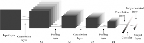
Among deep learning (DL) algorithms, the CNN is a feedforward neural network good at learning multi-dimensional matrix inputs. The CNN structure can be diversified by changing the combination between convolution and pooling layers. The structure of the traditional CNN is illustrated in Figure 1.
Figure 1. The structure of the traditional CNN
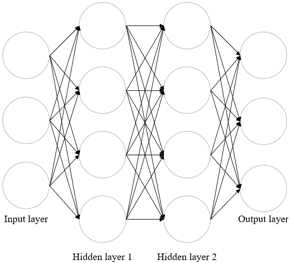
Figure 2. The connections between different layers of the CNN
Figure 2 shows the connections between different layers of the CNN. The traditional neural network (NN) cannot effectively handle the index data of our EIS, for most data are non-Euclidean space data with irregular and nonuniform dimensions and structures. If the traditional NN is directly applied to such data, the output results cannot accurately reflect the memberships, correlations, or relative importance between indices.
Figure 3. The parameter values of the proposed CNN
To solve the problem, this paper designs a CNN specifically for the evaluation of comprehensive HR quality of financial enterprises. The designed network can effectively classify the evaluation results based on the structure of the EIS. Figure 3 presents the parameter values of the proposed network.
Then, the convolution layers in Figure 3 were optimized in details. The index data Cij and N-index convolution can be calculated by:
${{C}_{ij}}{{*}_{G }}CON={{U}_{C{{K}_{\phi }}}}{{H}^{T}}{{C}_{ij}}$ (21)
where, CKφ is the convolution kernel of the CNN:
$C{{K}_{\phi }}=\sum\limits_{p=0}^{P}{{{\phi }_{p}}{{\Psi }^{p}}}$ (22)
where, ψp is the diagonal matrix composed of eigenvalues; φp is the kernel coefficient. After N-index convolution, the index data Cij can be expressed as:
$u=H\left( \sum\limits_{p=0}^{P}{{{\phi }_{p}}{{\Psi }^{p}}} \right){{H}^{T}}{{C}_{ij}}$ (23)
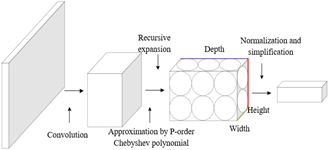
where, φp is the parameter matrix to be learned by the CNN. To minimize the computing load and complexity of the kernel, the kernel can be approximated by P-order Chebyshev polynomial:
$C{{K}_{\phi }}=\sum\limits_{p=0}^{P}{{{\phi }_{p}}{{Q}_{p}}\left( \frac{2\Psi }{{{\tau }_{max}}}-{{I}_{N}} \right)}$ (24)
where, φp is the coefficient of the P-order Chebyshev polynomial. The recursive expansion of the polynomial can be expressed as:
${{Q}_{p}}\left( {{C}_{ij}} \right)=2{{C}_{ij}}\cdot {{Q}_{p-1}}\left( {{C}_{ij}} \right)-{{Q}_{p-2}}\left( {{C}_{ij}} \right)$ (25)
Taking the initial term Q0(Cij) as1, then Q1(Cij)=Cij. Formula (25) can be redescribed by the recursively expanded polynomial as:
$\begin{align} & u=H\left( \sum\limits_{p=0}^{P}{{{\phi }_{p}}{{Q}_{p}}\left( \frac{2\Psi }{{{\tau }_{max}}}-{{I}_{N}} \right)} \right){{H}^{T}}{{C}_{ij}} \\ & =\sum\limits_{p=0}^{P}{{{\phi }_{p}}{{Q}_{p}}\left( {\hat{\Gamma }} \right)}{{C}_{ij}}=\sum\limits_{p=0}^{P}{{{\phi }_{p}}{{Q}_{p}}\left( \frac{2\Gamma }{{{\tau }_{max}}}-{{I}_{N}} \right)}{{C}_{ij}} \\\end{align}$ (26)
The above formula eliminates the multiplication with matrix H, thereby simplifying the calculation. Let the values of P and τmax be 2. Formula (27) can be simplified as:
$u={{\phi }_{0}}{{C}_{ij}}+{{\phi }_{1}}\left( \Gamma -{{I}_{N}} \right){{C}_{ij}}$ (27)
Then, the Laplace matrix can be normalized by:
${{\Gamma }^{*}}={{U}^{-{1}/{2}\;}}\Gamma {{U}^{-{1}/{2}\;}}={{I}_{N}}-{{U}^{-{1}/{2}\;}}L{{U}^{-{1}/{2}\;}}$ (28)
Substituting formula (28) to formula (27):
$u={{\phi }_{0}}{{C}_{ij}}+{{\phi }_{1}}\left( {{U}^{-{1}/{2}\;}}L{{U}^{-{1}/{2}\;}} \right){{C}_{ij}}$ (29)
If φ0 equals -φ1=θ, the above formula can be further simplified as:
$u=\left( {{I}_{N}}+{{U}^{-{1}/{2}\;}}A{{U}^{-{1}/{2}\;}} \right){{C}_{ij}}$ (30)
Then, the N-index convolution can be computed by:
$C_{ij}^{p+1}=\Phi \left( LC_{ij}^{p}{{\phi }^{p}} \right)$ (31)
where, L=IN+U-1/2AU-1/2; Cijp is the N×M-dimensional input of layer p (i.e. the input of each layer has N nodes, each has M-dimensional features); φp is the M×W-dimensional parameter matrix of layer p. M and W are the feature dimensions of input and output nodes in convolution layer, respectively. Hence, the output dimension of layer p+1 equals N×W. The workflow of N-index convolution is explained in Figure 4.
Figure 4. The workflow of N-index convolution
Under the cumulative effect of multiple convolutions, the eigenvalues generated in the two nearest matrices will be relatively large, resulting in vanishing gradients. To ensure the credibility of the evaluation results, L was renormalized by:
$\hat{L}={{\hat{U}}^{-{1}/{2}\;}}{{A}^{*}}{{\hat{U}}^{-{1}/{2}\;}}$ (32)
where, A*=λIN+W (IN is a self-connected identity matrix). Each node l can be calculated by:
$C_{ij}^{p+1}=\Phi \left( \sum\limits_{k\in {{N}_{l}}}{\frac{1}{{{\sigma }_{lk}}}C_{ij}^{p+1}}{{\phi }^{p}} \right)$ (33)
where, Nl is the set of neighboring nodes of node l; σij is the connection weight between nodes l and k. Figure 5 shows the update method of node l.
Figure 5. The update method of node l
Before training the proposed DNN, the sample data on all indices must be preprocessed, such that the training data are of the same dimension and order. The simulation software MATLAB offers three preprocessing methods: standardization, normalization, and principal component analysis (PCA). This paper selects the normalization with mapminmax function, which converts the data on each index into a number in (0, 1). To verify the effectiveness of our network, the parameters of the proposed CNN was configured as per Figure 3, and trained by the normalized index data.
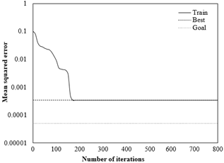
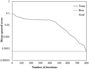
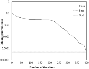
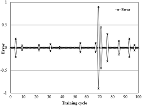
First, the CNN falling into the local minimum trap was verified by the index data. As shown in Figure 6, four groups of data had obvious bias in the verification. To overcome the local minimum trap and ensure the training stability, the original CNN was optimized by adding the N-index convolution, considering the improvement of comprehensive HR quality. Figure 7 compares the training error curves of the original CNN and the optimized CNN.
As shown in Figure 7, the original CNN converged better than the preset expected error after 800 iterations. The mean squared error was reduced to 5.214*10-5, indicating that the evaluation accuracy is desirable. The optimized CNN also achieved ideal evaluation accuracy. Only 3 test data were abnormal in the 100 iterations. The errors of the other index data were all controlled within the preset error range. To sum up, the proposed model can evaluate the comprehensive HR quality of financial enterprises in an accurate manner.
To verify its application effect, the trained CNN was tested on 200 index data. Table 2 compares some of the actual and expected outputs of comprehensive HR quality. It can be seen that the actual outputs were close to the expected outputs. Thus, our model can effectively evaluate the comprehensive HR quality of financial enterprises.
Figure 8 compares the comprehensive HR qualities evaluated by the original and optimized CNNs. Obviously, the optimized CNN, which integrates N-index convolution, achieved smaller error than the original CNN, and accurately evaluated the comprehensive HR quality. Through repeated simulation trainings, our model was proved to have advantages like small test error and strong stability.
Figure 6. The training error curve of the CNN falling into local minimum trap
(a) Original CNN
(b) Optimized CNN
Figure 7. The comparison of training error curves
Table 2. The comparison between actual and expected outputs of comprehensive HR quality
|
Serial number of index data |
Actual outputs |
Expected outputs |
||||||
|
1 |
0.9989 |
0.0011 |
0.0009 |
0.0008 |
1 |
0 |
0 |
0 |
|
2 |
0.0016 |
0.9952 |
-0.0023 |
-0.0033 |
0 |
1 |
0 |
0 |
|
3 |
0.0017 |
0.9998 |
-0.0013 |
-0.0015 |
0 |
1 |
0 |
0 |
|
4 |
0.0001 |
0.0010 |
1.0003 |
-0.0021 |
0 |
0 |
1 |
0 |
|
5 |
-0.0004 |
0.0021 |
1.0010 |
-0.0016 |
0 |
0 |
1 |
0 |
|
6 |
0.9998 |
0.0007 |
0.0005 |
0.0010 |
1 |
0 |
0 |
0 |
|
7 |
-0.0002 |
-0.0003 |
0.0002 |
1.0020 |
0 |
0 |
0 |
1 |
|
8 |
-0.0006 |
0.0017 |
1.0006 |
-0.0023 |
0 |
0 |
1 |
0 |
|
9 |
0.0028 |
0.9999 |
-0.0012 |
-0.0008 |
0 |
1 |
0 |
0 |
|
10 |
-0.0008 |
0.0009 |
1.0012 |
-0.0009 |
0 |
0 |
1 |
0 |
(a) Original CNN
(b) Optimized CNN
Figure 8. The comparison of evaluation results on comprehensive HR quality
This paper puts forward a DNN-based evaluation model for comprehensive HR quality of financial enterprises. Firstly, the authors constructed an EIS of 5 primary indices and 21 secondary indices, and decomposed the complex evaluation problem by layers and indices. Then, the improvement of comprehensive HR quality was introduced into the evaluation through the design of a CNN with N-index convolution. The experimental results show that the proposed network converged after 800 iterations, and its error fell within the preset error range. This means our network achieved a desirable evaluation effect. In addition, the actual outputs of our network were found close to the expected outputs. Therefore, the proposed CNN can effectively evaluate the comprehensive HR quality of financial enterprises.
[1] Jabbour, C.J.C., Sarkis, J., de Sousa Jabbour, A.B.L., Renwick, D.W.S., Singh, S.K., Grebinevych, O., Kruglianskas, I., Godinho Filho, M. (2019). Who is in charge? A review and a research agenda on the ‘human side’of the circular economy. Journal of Cleaner Production, 222: 793-801. https://doi.org/10.1016/j.jclepro.2019.03.038
[2] Guerci, M., Carollo, L. (2016). A paradox view on green human resource management: Insights from the Italian context. The International Journal of Human Resource Management, 27(2): 212-238. https://doi.org/10.1080/09585192.2015.1033641
[3] Haddock-Millar, J., Sanyal, C., Müller-Camen, M. (2016). Green human resource management: a comparative qualitative case study of a United States multinational corporation. The International Journal of Human Resource Management, 27(2): 192-211. https://doi.org/10.1080/09585192.2015.1052087
[4] Hecklau, F., Orth, R., Kidschun, F., Kohl, H. (2017). Human resources management: Meta-study-analysis of future competences in Industry 4.0. In Proceedings of the International Conference on Intellectual Capital, Knowledge Management & Organizational Learning, pp. 163-174.
[5] Kim, K., Shin, T.H. (2019). Additive effects of performance-and commitment-oriented human resource management systems on organizational outcomes. Sustainability, 11(6): 1679. https://doi.org/10.3390/su11061679
[6] López-Fernández, M., Romero-Fernández, P.M., Aust, I. (2018). Socially responsible human resource management and employee perception: The influence of manager and line managers. Sustainability, 10(12): 4614. https://doi.org/10.3390/su10124614
[7] Newman, A., Miao, Q., Hofman, P.S., Zhu, C.J. (2016). The impact of socially responsible human resource management on employees' organizational citizenship behaviour: the mediating role of organizational identification. The international journal of human resource management, 27(4): 440-455. https://doi.org/10.1080/09585192.2015.1042895
[8] Ogbeibu, S., Emelifeonwu, J., Senadjki, A., Gaskin, J., Kaivo-oja, J. (2020). Technological turbulence and greening of team creativity, product innovation, and human resource management: Implications for sustainability. Journal of Cleaner Production, 244: 118703. https://doi.org/10.1016/j.jclepro.2019.118703
[9] Opatha, H.H.D.N.P. (2019). A study of bachelor's degrees in human resource management in Three Sri Lankan Leading State Universities. Universal Journal of Educational Research, 7(11): 2361-2371. https://doi.org/10.13189/ujer.2019.071114
[10] Piwowar-Sulej, K. (2016). Flexibility in the Context of Project Teams' Human Potential. Przegląd Organizacji, (6): 48-54.
[11] Piwowar-Sulej, K., Bąk-Grabowska, D. (2018). Enterprise boundaries in the area of human resources. Argumenta Oeconomica, 2(41): 357-359. https://doi.org/10.15611/aoe.2018.2.16
[12] Singh, S.K., Del Giudice, M., Chierici, R., Graziano, D. (2020). Green innovation and environmental performance: The role of green transformational leadership and green human resource management. Technological Forecasting and Social Change, 150: 119762. https://doi.org/10.1016/j.techfore.2019.119762
[13] Delery, J., Gupta, N. (2016). Human resource management practices and organizational effectiveness: internal fit matters. Journal of Organizational Effectiveness: People and Performance, 3(2): 139-163. https://doi.org/10.1108/JOEPP-03-2016-0028
[14] Wang, X.L., Wang, L., Bi, Z., Li, Y.Y., Xu, Y. (2016). Cloud computing in human resource management (HRM) system for small and medium enterprises (SMEs). The International Journal of Advanced Manufacturing Technology, 84: 485-496. https://doi.org/10.1007/s00170-016-8493-8
[15] de Brito, R.P., de Oliveira, L.B. (2016). The relationship between human resource management and organizational performance. Brazilian Business Review, 13(3): 90-110. https://doi.org/10.15728/bbr.2016.13.3.5
[16] Crowley, F., Bourke, J. (2017). The influence of human resource management systems on innovation: Evidence from Irish manufacturing and service firms. International Journal of Innovation Management, 21(1): 1750003. https://doi.org/10.1142/S1363919617500037
[17] Ali, M. (2016). Impact of gender-focused human resource management on performance: The mediating effects of gender diversity. Australian Journal of Management, 41(2): 376-397. https://doi.org/10.1177/0312896214565119
[18] McClean, E., Collins, C.J. (2019). Expanding the concept of fit in strategic human resource management: An examination of the relationship between human resource practices and charismatic leadership on organizational outcomes. Human Resource Management, 58(2): 187-202. https://doi.org/10.1002/hrm.21945
[19] O'Donohue, W., Torugsa, N. (2016). The moderating effect of ‘Green’HRM on the association between proactive environmental management and financial performance in small firms. The International Journal of Human Resource Management, 27(2): 239-261. https://doi.org/10.1080/09585192.2015.1063078
[20] Rekalde, I., Landeta, J., Albizu, E., Fernandez-Ferrin, P. (2017). Is executive coaching more effective than other management training and development methods? Management Decision, 55(10): 2149-2162. https://doi.org/10.1108/MD-10-2016-0688
[21] Singh, S.K., Del Giudice, M., Tarba, S.Y., De Bernardi, P. (2019). Top management team shared leadership, market-oriented culture, innovation capability, and firm performance. IEEE Transactions on Engineering Management. https://doi.org/10.1109/TEM.2019.2946608
[22] Kelliher, C., Johnson, K. (1997). Personnel management in hotels - an update: a move to human resource management?. Progress in Tourism and Hospitality Research, 3(4): 321-331. https://doi.org/10.1002/(SICI)1099-1603(199712)3:4<321::AID-PTH109>3.0.CO;2-B
[23] Stone, D.L., Deadrick, D.L., Lukaszewski, K.M., Johnson, R. (2015). The influence of technology on the future of human resource management. Human Resource Management Review, 25(2): 216-231. https://doi.org/10.1016/j.hrmr.2015.01.002
[24] Burke, R.J. Spurgeon, P., Cooper, C.L. (2012). The innovation imperative in health care organisations: Critical role of human resource management in the cost, quality and productivity equation. New Horizons in Management series. Cheltenham: Edward Elgar Publishing.
[25] Lu, K., Zhu, J., Bao, H. (2015). High-performance human resource management and firm performance. Industrial Management & Data Systems, 115(2): 353-382. https://doi.org/10.1108/IMDS-10-2014-0317