Jyostna Devi Bodapati* | Annepu Vijay | Naralasetti Veeranjaneyulu
© 2020 IIETA. This article is published by IIETA and is licensed under the CC BY 4.0 license (http://creativecommons.org/licenses/by/4.0/).
OPEN ACCESS
Tumor grown in the human brains is one of the significant reasons that lead to loss of lives globally. Tumor is malignant collection of cells that grow in the human body. If these tumors grow in the brain, then they are called as brain tumors. Every year large number of human lives are lost due to this disease. Early detection of the disease might save the lives but requires experienced clinicians and diagnostic procedure that requires time and is very expensive. Therefore, there is a requirement for a robust system that automates the process of tumor identification. The idea behind this paper is to diagnose brain tumors by identifying the affected regions from the brain MRI images using machine learning approaches. In the proposed approach, prominent features of the tumor images are collected by passing them through a pre-trained Convolutional Network, VGG16. We observe that SVM gives better accuracy than other models. Though we achieve 84% accuracy, we feel the performance is not satisfactory. To make the model more robust, we obtain the most discriminant features, by applying Linear Discriminant Analysis (LDA) on the features obtained from VGG16. We use different conventional models like logistic regression, K-Nearest neighbor classifier (KNN), Perceptron learning, Multi Layered Perceptron (MLP) and Support Vector Machine (SVM) for the comparison study of the tumor image classification task. The proposed model leads to an accuracy of 100% as deep features extract important characteristics of the data and further LDA projects the data onto the most discriminant directions.
brain tumor detection, linear transformation, transfer learning, latent space, radial basis kernel (RBF), linear kernel, glioma detection, deep neural features
Unusual cell growth in the human body is referred to as a Tumor. Tumors that grow in the brain or spinal cord are referred to as brain tumors. Tumors can either be benign or malignant. Tumors that spread to other body parts are called as malignant while those that will not spread are called as benign. Malignant tumors are harmful than benign tumors as they invade other parts of brain. Though benign tumors do not invade other parts they are still harmful as they cause problems by pressing other tissues of the brain. Hence early detection of these tumors helps to save lives. Brain tumor, statistically, is the 10th leading cause of deaths in both men and women [1]. Every year thousands of people suffer and evade their lives due to these brain tumors.
Diagnosis of Brain cancer involves Physical examination of MRI, X-Ray or CT scan. Among all the possible methods, diagnosis through MRI images is the most reliable and safest method as it does not involve exposing the body to any sort of harmful radiation. Given the MRI image, it is required to identify whether the tumor is present or not in the image. Once the tumor is confirmed then finding the location and size of the tumor is required. Doing this manually requires experts in the domain, time taking and expensive moreover it is prone to errors. Hence manually doing this is not effective and automation would be very much helpful to clinicians to identify the tumors in the brain. In this work, we introduce a simple tool based on machine learning to identify presence or absence of tumors in the MRI scan of the human brain. Focus of this work is on predicting the presence or absence of the tumor not on the segmentation part.
Since the introduction, numerous techniques that leverage machine learning have been introduced for tumor identification and detection. Majority of work in the literature focuses on deciding whether a tumor is present or not in the given image. Once the tumor is confirmed then the objective could be classifying the type of tumors [2-5]. Another line of research after tumor confirmation could be to find the location of the tumor and segment it [6-9]. There are few methods that can do both identification of the tumor and then segmenting the affected parts [10, 11].
Though there are a good number of methods available in the literature, all of them are either suboptimal or complex. In this paper we focus on designing a simple, optimal and robust model for detecting the tumor as early as possible given the MRI image of brain by leveraging existing machine learning algorithms. In the proposed approach, prominent features of the brain MRI image are collected by passing them through a pre-trained ConvNet, VGG16. According to the literature, VGG16 features give state of the art results for classification of the given images [12], hence we extract deep features of the given MRI image using pre-trained VGG16 model. The features extracted from VGG16 are used to learn a model that automates the process of tumor Screening. We used different conventional and simple models [13, 14] like logistic regression, K-Nearest neighbor classifier (KNN), Perceptron learning, Multi-Layer feed forward neural network (MLFFNN) and Support Vector Machine (SVM) [15] for comparative studies. We observe that SVM gives better accuracy among the other models. Though the existing methods give 84% accuracy, the performance is not satisfactory. To improve the performance further, we apply linear transformation on the data. The directions for projections are obtained by using Linear Discriminant Analysis (LDA). Deep features extracted from pretrained CNN (VGG16) are projected in the most discriminant directions to obtain the most discriminant features [16]. These projected features are used for training the model that in turn leads to an optimal model with an accuracy of 100%. That proposed model gives zero error on the test data though it is simple without any complex structures.
Following are the major contributions of the proposed work:
· Design a simple yet optimal and robust classifier for recognizing the presence of tumor in brain MRI images
· Usage of deep features to get important characteristics of the MRI image
· Use linear projections to reduce the number of features while preserving discrimination information
In the beginning of this section, we present the conventional models available in the literature for brain tumor classification. Then we will present a detailed study of deep learning-based models for the same task.
This part of this section gives taxonomy of conventional models available in the literature for the task of tumor identification [2-5, 7, 17, 18]. Multiple approaches on detection and classification of the type of tumors [2-5, 18]. Another set of methods focus on segmenting the region of interest after detecting the tumor [7, 17].
Gabor filters are used to extract texture-based features from the images [2]. To avoid over-fitting, unwanted feature elimination is done by feature selection methods like rank-based methods and recursive feature elimination methods. SVM based recursive feature elimination approach is used to retain important features and to eliminate unwanted features from the data. This model is compared with the standard dimensionality reduction techniques like constrained LDA.
The problem of tumor classification is treated as a voxel classification task as the voxel class is dependent on their neighboring voxels [3]. Conditional random field (CRF) methods are used to represent spatial relationships among the voxels.
Various filters have been applied to remove noise from the images [4], then wavelet features are extracted and finally the images are classified using support vector-based classification methods.
Feature selection methods (wrapper based) are used to extract important features from the features extracted from regions of interest [5]. KNN classifier is used to discriminate low grade neoplasm to high grade neoplasms.
Alignment-based features are used to fragment the tumor affected region from the given brain tumor images [7]. Four different types of alignment-based features, intensity and spatial normalized images, normal tissue spatial priors, expected intensity spatial maps and smoothed spatial brain mask and left to right symmetry have been considered in this work. The quality of segmentation is measured by Jaccard similarity measure.
DCT features are extracted from the given CT scan images and the Bayesian classification model is used to identify whether tumor is present in the given image or not [17]. If the initial test gives a positive result (means tumor exists) then to extract the tumor part, simple k-means algorithm is applied. An SVM based classification is proposed that uses LBP features extracted from the MRI images [18].
In the next part of this section we present different deep learning models [9, 11, 19, 20-22] that are available in the literature. Few works [9, 20-22] focus on either detection of classification or classification of the type of tumors. The region of image is segmented before image is being classified [8, 11, 19].
A fully convolutional neural network (FCNN) with Continuous random filed (CRF) is proposed by Zhao et al. [9] to segment the affected region from the given image. DWT based features are extracted, and deep learning models are used as classification methods to identify the type of tumor [20].
A convolution neural network-based method is proposed to grade tumor type and the kernels at different layers of the trained CNN have been reported for visualization [21]. A CNN based segmentation method is proposed. They claim that small size kernels like 3 x 3 size works better than other kernel sizes as they allow deeper architectures [22].
A deep learning-based approach has been proposed [19]. C-means clustering, a fuzzy technique is used to slice the tumor part. Initially, tumor part is segmented, and features are extracted using DWT and then for dimensionality reduction (Principal component analysis) PCA is applied over the features to avoid over-fitting. Finally, a deep architecture is trained to classify the data.
To segment the tumor part from the given MRI images they proposed a deep learning-based method [8]. This deep learning network can extract both local as well as global contextual features simultaneously. Different deep learning-based techniques and models were studied focusing on both segmentation and classification [11].
Most of the existing methods use conventional models for classification and hand-crafted features for feature extraction. Few other methods use deep features that are learned as part of the deep model that is used for classification. In case of former models, the model is not robust and in the latter case, the models are robust, but we need large datasets. Our objective is to create a simple and robust model with limited dataset and with limited computational power. To achieve our objective, we use deep models that are pre-trained on large datasets to extract features and conventional models to classify the given brain tumor images. To further improve the performance of the models, we reduced the dimensionality of the data using linear projections. As the features are reduced the models are immune to over-fit and robust.
We propose a simple and robust machine learning based approach to identify the severity level of tumor in brain based on their MRI images. In the proposed method we do not need much pre-processing of the training data which reduces the time during testing. Instead of applying complex pre-processing steps we extract the features that are most descriptive.
Hand crafted features like gist, hog and sift gives global or local representation of the image. Till the entry of deep learning models, the hand-crafted features were dominant and being widely used for feature extraction. Deep learning models do not require hand crafted features as the models themselves can learn the important characteristics of the input images. This special capability of the deep models makes them representation models, as these models can represent the data efficiently. This reduces the conventional feature extraction phase where features are handcrafted. But the downside of the deep learning models is that they need enormous amounts of data for training, which is usually scarce for most of the real-time applications. This problem is addressed by the introduction of transfer learning where the knowledge gained by a deep learning model can be transferred to other models without any training. For example, use pre-trained models like VGG16 to extract features from the given input image.
Pre-trained models are the models that are trained on large amounts of data and the weights updated during the training of the complex model can be applied for similar tasks. VGG16 is one of the pre-trained models that achieve an accuracy of 92.7% on 14 million image dataset with 1000 different classes. Deep models like VGG16, VGG19, ResNet152, InceptionV3 when used for feature extraction are proved to be better than the hand-crafted features as these models can represent the images efficiently.
The complete architecture is divided into 3 different modules named pre-processing, feature extraction and model training and evaluation (Figure 1).
Pre-processing Module: The MRI images of the dataset are of varying sizes. During the pre-processing stage we resize the images of the dataset so that all the images in the entire dataset will be of the same size.
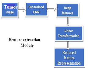
Feature extraction Module: During this phase, pre-trained model VGG16 is used to get 4096 deep features. The reason for the poor performance of any machine learning model could be the improper bias and variance. One way to avoid model over-fitting is by reducing the number of dimensions of the data. After extracting deep features fromVGG16, to avoid the curse of dimensionality problem we apply linear dimension reduction techniques. Principal component analysis is one of the feature transformation methods, where the features are projected to some other space without loss. In PCA, the data is projected onto the directions of maximum variance. If the class separability information is not preserved after projection, then the performance of the model degrades. LDA addresses this issue by projecting the data onto the directions of max separability. Hence, we prefer LDA to PCA and kernel PCA (KPCA) for data projection in lower dimension space. In this module, we extract deep features and apply linear transformation to reduce the number of dimensions while preserving the class separability information in the data. Figure 2 shows the application of linear transformation as a supervised model. Figure 3(a) shows the detailed architecture of the proposed module.
Figure 1. Architecture of the proposed system
Figure 2. Supervised linear transformation of data
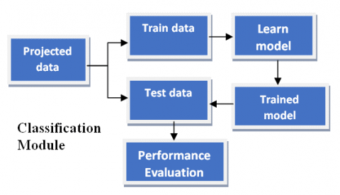
Model training and evaluation module: During this phase, we train the model on trained data that is formed using the features in the transformed space, apply the model on test data, evaluate the model performance on test data. Figure 3(b) shows the details of this module.
The proposed model is simple as the model can be any shallow model and the model is robust as the features we extract from the deep pre-trained models. As the model is trained on large volumes of data, the features we extract are much more efficient. As we need not train any deep model, we do not need large volumes of data for training, neither long time nor enormous computing resources during the model training.
(a)
(b)
Figure 3. (a) Feature extraction module (Upper), (b) Model training and evaluation module (Bottom)
Pseudo code for the proposed algorithm: Initially the given brain MRI images are preprocessed, then features are extracted using pretrained model. Then the deep features are projected using one of the projection techniques and then classified. Table 1 shows the proposed algorithm.
|
Let the data for training be {(x1,y1), ....(xn, yn)}, where each xi ϵ Rd and yi ϵ{0,1}. Step 1: Preprocess the images such that all the images in the dataset will be of the same size. For each xi in training data apply crop function to bring all the images to the size 224 x 224 x 3. Step 2: Load VGG16 pre-trained model and remove the final classification layer, for each example in the training data feed to VGG16 (without) and get the deep features. For each image xi in the training dataset get 4096 features Step 3: Apply linear transformation to reduce the dimensions in the most discriminant directions. We use LDA to transform the data to reduced space. Following are the steps involved in LDA transformation:
$S_{i}=\sum_{\mathrm{x} \in \omega_{\mathrm{i}}}\left(\mathrm{x}-\mu_{\mathrm{i}}\right)\left(\mathrm{x}-\mu_{\mathrm{i}}\right)^{\mathrm{T}}$
$S_{B}=\left(\mu_{\mathrm{i}}-\mu\right)\left(\mu_{\mathrm{i}}-\mu\right)^{T}$
Step 4: Train a model on the reduced dimensional representation (x’); performance of the SVM model is evaluated on test data. The primal objective function of SVM is: $L\left(w, w_{0}\right)=\min \left[w^{T} w-\sum_{i=1}^{n} \propto_{i}\left[y_{i}\left(w^{T} x_{i}+w_{0}\right)-1\right]\right.$ where, $\propto_{1}, \dots, \propto_{n}$ . The dual objective function of SVM is: $L\left(\propto_{1}, \ldots \propto_{n}\right)=\frac{1}{2} \sum_{i=1}^{n} \sum_{j=1}^{n}\left(\propto_{i} \propto_{j} y_{i} y_{j}\left(x_{i}^{T} x_{i}\right)\right)+\sum_{j=1}^{n} \alpha_{i}$ Subject to the condition that $\sum_{j=1}^{n} \propto_{i} y_{i}=0$ and $\propto_{1}, \dots, \propto_{n}$ . SVM basically gives linear boundary to get a non- linear boundary we can use kernel functions. The dual objective function of SVM with kernel functions is: $L\left(\propto_{1}, \ldots \propto_{n}\right)=\frac{1}{2} \sum_{i=1}^{n} \sum_{j=1}^{n}\left(\propto_{i} \propto_{j} y_{i} y_{j} K\left(x_{i}^{T} x_{i}\right)\right)+\sum_{j=1}^{n} \propto_{i}$ Step 5: After training the model on train data use the trained model on test data to get the performance measure. We use accuracy as the measure: Accuracy = $\frac{T P+T N}{N}$ TP (True Positives): Presence of tumor is correctly identified TN (True Negatives): Absence of tumor is correctly identified. N: Total number of examples |
Table 1. Proposed algorithm for Glioma detection
|
Kernel type |
Computation |
|
Linear kernel |
K(xm, xn) = a+b xmTxn |
|
Sigmoid kernel |
K(xm, xn) = tanh(xmTxn + θ) |
|
Polynomial kernel |
K(xm, xn) = (a xmTxn + b)d |
|
Gaussian kernel |
K(xm, xn) = exp( - $\frac{\| x_{m}-x_{n \|}}{2 \sigma^{2}}$ ) |
In this section, the results of various experiments we have performed to understand the efficiency of our proposed method are presented. First, we introduce the dataset used for our studies followed by the detailed presentation of results of the proposed model for automatic brain tumor recognition based on MRI images.
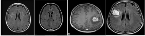
Summary of the dataset: To prove the efficiency of the proposed model and for the experimental studies we have used the benchmark dataset available at Kaggle [23]. The dataset contains a set of MRI images taken under variety of imaging conditions. The images are rated manually either as tumor exists or as non-tumor images, indicating either the presence or the absence of tumor respectively. The dataset has a total of 253 MRI images belonging to both affected and not affected images. Out of the total images, 155 images are affected while 98 images are non-tumor images.
Figure 4 shows few sample images from the kaggle dataset with tumor and without tumor.
Table 2. Summary of the tumor dataset
|
Number of Total images |
253 |
|
Number of Tumor images |
155 |
|
Number of Non-Tumor images |
98 |
|
Number of pixels in image |
2622 |
|
Number of Train Images |
203 |
|
Number of Test Images |
50 |
Figure 4. Sample images from the dataset without tumor (left 2 images) and with tumor (right 2 images)
Experiment - Check the brain MRI contains a tumor or not: The objective here is to identify whether there exists any tumor or not in the given MRI image. As there are only two classes, the task is a binary classification task. Our proposed model is applied on the given dataset in order to prove its robustness.
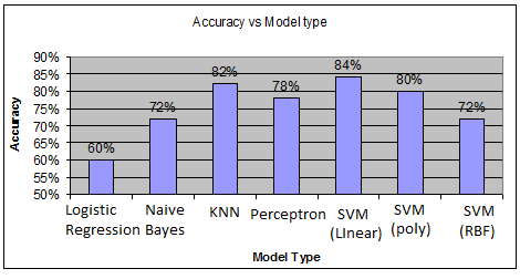
Various kernels used with SVM in the experiments are given in Table 2. From Table 3 and Figure 5 we can observe that SVM with linear kernel gives more accuracy than other models. Except logistic regression, rest of the models, perform better for this task with very few misclassifications. We observe that the data is linearly separable and applied LDA to project the data to reduced space.
Table 3. Performance of different classification models in deep feature space
|
Classification Model |
Accuracy |
|
|
Logistic Regression |
60% |
|
|
Naïve Baye’s |
72% |
|
|
K-Nearest Neighours (K-NN) |
82% |
|
|
Perceptron |
78% |
|
|
Support Vector Machine (SVM) |
Linear kernel |
84% |
|
Polynomial kernel |
80% |
|
|
Gaussian Kernel |
72% |
|
Figure 5. Performance of different classification models in deep feature space
Table 4. Performance of different classification models after applying different projections
|
Classification Model |
Accuracy after applying different projections |
|||
|
PCA |
KPCA |
LDA |
||
|
Logistic Regression |
84% |
58% |
100% |
|
|
Naïve Baye’s |
60% |
53% |
100% |
|
|
K-Nearest Neighours (KNN) |
76% |
58% |
100% |
|
|
Perceptron |
88% |
61% |
100% |
|
|
Support Vector Machine (SVM) |
Linear kernel |
80% |
78% |
100% |
|
Polynomial kernel |
78% |
85% |
100% |
|
|
Gaussian Kernel |
65% |
85% |
96% |
|
From Table 4 we can observe that the models have become more robust in the reduced feature space. The reason for this could be the data is projected to the space where it is linearly separable. Especially when the data is projected using LDA the data became linearly separable hence the model classifies the data without any errors.
Based on the results shown in Table 3 and Figure 6 we can observe that all the models (except SVM with kernel) classify the data with 0 error when the data is projected using LDA. Parameters used for SVM are g=0.2 and c=1000. SVM with RBF kernel misclassifies few examples but the reason could be bad width parameter.
Figure 6. Performance of the model in different reduced spaces
Figure 7. Deep features of MRI image data projected onto 1D
Figure 7 shows the image data after projecting the data to 1-D. As the data is linearly separable in 1D even simple linear models like logistic regression and KNN classifies the data without any misclassifications.
Table 5. Performance of SVM with different number of projections using PCA
|
Dimensions for projection (K) |
5 |
12 |
50 |
62 |
81 |
100 |
201 |
|
Accuracy |
88% |
78% |
88% |
88% |
84% |
80% |
82% |
In Table 5, K value indicates the number of directions used for projection using PCA. Using PCA we can project the data from 1 to maximum number of features. We have varied the number of projections from 1 to 201 directions. With just 5 dimensions SVM gives 88% accuracy. The reason for the high performance of the proposed model could be the features and the directions of projection. The features we get are the best features from deep CNN and then to avoid over-fitting of the models we project the data in the directions of the maximum separability.
The objective of our work is to develop a model that can automatically predict the existence of brain tumor from given MRI images. Our proposed model is simple yet robust. Initially deep features are extracted from pre-trained VGG16 to represent the more prominent features from the brain MRI images. To avoid over-fitting of the model the extracted deep features are projected to reduced dimensions while preserving the class discriminant information. Based on the experiments, we claim that when deep features are projected, performance of the classification models improve. LDA based projection gives robust performance than other projections. The power of deep learning and simplicity of the models make the model more robust. Hence the proposed model classifies the tumor images without any misclassifications.
[1] Stephanie, S., Brix, T., Varghese, J., Warneke, N., Schwake, M., Brokinkel, B., Ewelt, C., Dugas, M., Stummer, W. (2019). Adverse events in brain tumor surgery: Incidence, type, and impact on current quality metrics. Acta Neurochirurgica, 161: 287-306. https://doi.org/10.1007/s00701-018-03790-4
[2] Zacharaki, E.I., Wang, S.M., Chawla, S., Yoo, D.S., Wolf, R., Melhem, E.R., Davatzikos, C. (2009). Classification of brain tumor type and grade using MRI texture and shape in a machine learning scheme. Magnetic Resonance in Medicine: An Official Journal of the International Society for Magnetic Resonance in Medicine, 62(6): 1609-1618. https://doi.org/10.1002/mrm.22147
[3] Bauer, S., Nolte, L.P., Reyes, M. (2011). Fully automatic segmentation of brain tumor images using support vector machine classification in combination with hierarchical conditional random field regularization. International Conference on Medical Image Computing and Computer-Assisted Intervention, Springer, Berlin, Heidelberg, pp. 354-361.
[4] Gurusamy, R., Subramaniam, V. (2017). A machine learning approach for MRI brain tumor classification. Computers, Materials & Continua, 53(2): 91-108. https://doi.org/10.3970/cmc.2017.053.091
[5] Zacharaki, E.I., Kanas, V.G., Davatzikos, C. (2011). Investigating machine learning techniques for MRI-based classification of brain neoplasms. International Journal of Computer Assisted Radiology and Surgery, 6: 821-828. https://doi.org/10.1007/s11548-011-0559-3
[6] Zhou, J., Chan, K.L., Chong, V.F.H., Krishnan, S.M. (2006). Extraction of brain tumor from MR images using one-class support vector machine. 2005 IEEE Engineering in Medicine and Biology 27th Annual Conference, Shanghai, China. https://doi.org/10.1109/IEMBS.2005.1615965
[7] Schmidt, M., Levner, I., Greiner, R., Murtha, A., Bistritz, A. (2005). Segmenting brain tumors using alignment-based features. Fourth International Conference on Machine Learning and Applications (ICMLA'05), Los Angeles, CA, USA. https://doi.org/10.1109/ICMLA.2005.56
[8] Havaei, M., Davy, A., Warde-Farley, D., Biard, A., Courville, A., Bengio, Y., Pal, C., Jodoin, P.M., Larochelle, H. (2017). Brain tumor segmentation with deep neural networks. Medical Image Analysis, 35: 18-31. https://doi.org/10.1016/j.media.2016.05.004
[9] Zhao, X.M., Wu, Y.H., Song, G.D., Li, Z.Y., Zhang, Y.Z., Fan, Y. (2018). A deep learning model integrating FCNNs and CRFs for brain tumor segmentation. Medical Image Analysis, 43: 98-111. https://doi.org/10.1016/j.media.2017.10.002
[10] Zhou, M., Scott, J., Chaudhury, B., Hall, L., Goldgof, D., Yeom, K.W., Iv, M., Ou, Y., Kalpathy-Cramer, J., Napel, S., Gillies, R., Gevaert, O., Gatenby, R. (2018). Radiomics in brain tumor: image assessment, quantitative feature descriptors, and machine-learning approaches. American Journal of Neuroradiology, 39(2): 208-216. https://doi.org/10.3174/ajnr.A5391
[11] Akkus, Z., Galimzianova, A., Hoogi, A., Rubin, D.L., Erickson, B.J. (2017). Deep learning for brain MRI segmentation: State of the art and future directions. Journal of Digital Imaging, 30(4): 449-459. https://doi.org/10.1007/s10278-017-9983-4
[12] Bodapati, J.D., Veeranjaneyulu, N. (2019). Feature extraction and classification using deep convolutional neural networks. Journal of Cyber Security and Mobility, 8(2): 261-276. https://doi.org/10.13052/jcsm2245-1439.825
[13] Jyostna Devi, B. (2019). Effect of different kernels on the performance of an SVM based classification. In International Journal of Recent Technology and Engineering (IJRTE), 7(5S4): 1-6.
[14] Bodapati, J.D., Krishna Sajja, V.R., Mundukur, N.B., Veeranjaneyulu, N. (2019). Robust cluster-then-label (RCTL) approach for heart disease prediction. Ingénierie des Systèmes d’Information, 24(3): 255-260. https://doi.org/10.18280/isi.240305
[15] Polisetty, K., Paidipati, K.K., Bodapati, J.D. (2019). Modelling of monthly rainfall patterns in the north-west india using SVM. Ingénierie des Systèmes d’Information, 24(4): 391-395. https://doi.org/10.18280/isi.240405
[16] Veeranjaneyulu, N., Raghunath, A., Jyostna Devi, B., Mandhala, V.N. (2014). Scene classification using support vector machines with LDA. Journal of Theoretical & Applied Information Technology, 63(3).
[17] Ain, Q.U., Mehmood, I., Naqi, S.M., Arfan Jaffar, M. (2010). Bayesian classification using DCT features for brain tumor detection. International Conference on Knowledge-Based and Intelligent Information and Engineering Systems. Springer, Berlin, Heidelberg. https://doi.org/10.1007/978-3-642-15387-7_38
[18] Deepika, K., Jyostna Devi, B., Ravu, K.S. (2019). An efficient automatic brain tumor classification using lbp features and SVM-based classifier. Proceedings of International Conference on Computational Intelligence and Data Engineering, Springer, Singapore. https://doi.org/10.1007/978-981-13-6459-4_17
[19] Mohsen, H., El-Dahshan, E.S.A., El-Horbaty, E.S.M., Salem, A.B.M. (2018). Classification using deep learning neural networks for brain tumors. Future Computing and Informatics Journal, 3(1): 68-71. https://doi.org/10.1016/j.fcij.2017.12.001
[20] Bodapati, J.D., Kishore, K.V.K., Veeranjaneyulu, N. (2010). An intelligent authentication system using wavelet fusion of K-PCA, R-LDA. International Conference on Communication Control and Computing Technologies, Ramanathapuram, India. https://doi.org/10.1109/ICCCCT.2010.5670591
[21] Pan, Y.H., Huang, W.M., Lin, Z.P., Zhu, W.Z., Zhou, J.Y., Wong, J., Ding, Z.X. (2015). Brain tumor grading based on neural networks and convolutional neural networks. 2015. 37th Annual International Conference of the IEEE Engineering in Medicine and Biology Society (EMBC), Milan, Italy. https://doi.org/10.1109/EMBC.2015.7318458
[22] Pereiraa, S., Pinto, A., Alves, V., Silva, C.A. (2016). Brain tumor segmentation using convolutional neural networks in MRI images. IEEE Transactions on Medical Imaging, 35(5): 1240-1251. https://doi.org/10.1109/TMI.2016.2538465
[23] https://www.kaggle.com/navoneel/brain-mri-images-for-brain-tumor-detection