Ge Wang | Junjie Wei | Banghua Yao*
© 2020 IIETA. This article is published by IIETA and is licensed under the CC BY 4.0 license (http://creativecommons.org/licenses/by/4.0/).
OPEN ACCESS
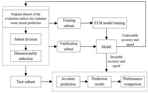
The prevention of water inrush is of great significance to the work safety in coalmines. However, the existing prediction models for coalmine water inrush cannot achieve desirable speed, accuracy, or generalization ability, owing to the complexity and diversity of causes of this accident. Therefore, this paper develops an artificial intelligence (AI)-based coalmine water inrush safety prediction model, making coalmine water inrush prediction more accurate, real-time, and robust. Firstly, the causes of coalmine water inrush were combed, and used to build a reasonable evaluation index system. Next, the extreme learning machine (ELM) was optimized with particle swarm optimization (PSO) algorithm and ant colony optimization (ACO) algorithm, and developed into a coalmine water inrush safety prediction model. The dimensionality reduction in subset classification was introduced in great details. Finally, the effectiveness of our model was proved through experiments. The research results provide the basis for the application of combinatory optimized learning machines in hazard prediction of other fields.
artificial intelligence (AI), extreme learning machine (ELM), coalmine water inrush prediction, particle swarm optimization (PSO) algorithm, ant colony optimization (ACO) algorithm
China boasts a wealth of coal resources. All varieties of coal have been detected in mines across the country. The supply of coal, the leading primary energy source, directly affects industrial development and even social stability [1-6]. Many coalmines in China face complex hydrogeological conditions. If a water inrush occurs, the roadway will be quickly flooded if the accident is not handled properly, posing a serious threat to the lives of workers and the safety of coalmine properties [7-9]. Therefore, the prevention of water inrush is recognized as the key to the work safety in coalmines. An effective way to prevent water inrush is to build a water inrush safety model for the target coalmine [10-12].
The causes of water inrush vary from mine to mine, because each coalmine has unique hydrogeological and storage conditions. Considering the variation, many scholars have explored the mechanism of coalmine water inrush, constructed evaluation index system of coalmine water inrush safety, and introduced artificial intelligence (AI) into the analysis and prediction of coalmine water inrush [13-16].
From the perspective of physics, Winkler [17] considered the defect and local instability of the rock floor as the main causes of coalmine water inrush, and proposed to judge the rock floor instability by detecting whether the stress of the water barrier is imbalanced. Kumari and Om [18] combined mathematics with structural mechanics, and systematically analyzed the causes of water inrush fault in coalmines, based on catastrophe theory and limit bending moment theory. Based on some coalmine water inrush samples, Henriques and Malekian [19] discretized the continuous water inrush prediction information with support vector machine (SVM), and solved the local minimum problem of traditional neural networks (NNs). Zhang et al. [20] combined the genetic algorithm (GA) with backpropagation (BP) algorithm into a coalmine water inrush prediction model based on artificial neural network (ANN); the model has a high training accuracy, but consumes too much time in adjusting the network parameters.
The prediction of coalmine water inrush must be rapid, accurate, and effective. Hence, it is important to improve the operating speed of the prediction model, while ensuring the prediction accuracy [21-23]. Bhattacharjee et al. [24] developed a hybrid prediction model based on extreme learning machine (ELM) and the principal component analysis (PCA), and proved that the hybrid model is more accurate and faster than the least squares (LS) SVM and traditional BP model. Liu et al. [25] constructed a real-time monitoring system for water inrush from coalmine floor, and optimized the input weights and hidden layer bias, which are assigned randomly by the ELM, with the adaptive difference algorithm.
Traditionally, the evaluation index systems for coalmine water inrush overlook the fact that the causes of water inrush might change in real time with external forces in coalmining. Moreover, the existing ELM-based prediction algorithms cannot achieve desirable classification accuracy or generalization, despite their rapid prediction. To solve these problems, this paper develops an AI-based coalmine water inrush safety prediction model, making coalmine water inrush prediction more accurate, real-time, and robust. Firstly, the causes of coalmine water inrush were combed, and a reasonable evaluation index system was established. Next, the feasibility of optimizing the ELM with particle swarm optimization (PSO) algorithm and ant colony optimization (ACO) algorithm was demonstrated, and the coalmine water inrush safety prediction model was created based on the ELM optimized by the PSO and ACO. The dimensionality reduction in subset classification was introduced in great details. Finally, the effectiveness and real-time performance of our model were proved through experiments.
Coalmine water inrush is the combined result of multiple factors, including but not limited to hydrogeological conditions, and human intervention. The cause of water inrush will change continuously, under the effect of the external forces in coalmining and single influencing factors.
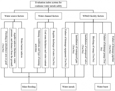
Referring to the existing evaluation index systems, this paper summarizes the factors affecting coalmine water inrush, and selects three primary indices for coalmine water inrush safety: water source factors, water channel factors, and factors of water-proof and drainage (WP&D) facilities. Specifically, the water source factors include three secondary indices: aquifer indices (thickness, water pressure, and distance from the ground), water barrier indices (e.g. thickness), and flooding in subsidence area or goaf (Yes/No); the water channel factors include three secondary indices: regular discharge of water (Yes/No), coal seam thickness and water content, and mining conditions and type of mining activities; the WP&D facility factors include six secondary indices: blocking of sump (Yes/No), installation of waterproof valve (Yes/No), installation of waterproof gate (Yes/No), failure of drainage pump (Yes/No), failure of drainage pipeline (Yes/No), and failure of drainage equipment (Yes/No). The proposed evaluation index system for coalmine water inrush safety is presented in Figure 1.
The complex influencing factors complicate the prediction of water inrush in coalmines. Fortunately, the correlations between these factors can be identified through AI technologies. Based on the proposed two-layer evaluation index system, this paper decides to build an ELM model to predict coalmine water inrush.
Figure 1. The proposed evaluation index system for coalmine water inrush safety
3.1 The ELM algorithm
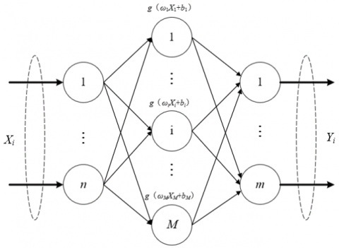
The ELM algorithm is a learning algorithm based on a feedforward NN with a single hidden layer (Figure 2). The most notable advantage of the algorithm is its fast speed, which arises from the fact that the algorithm can find the unique optimal solution from the generalized reverse by adjusting the number of nodes, without needing to change the input weights or biases of the hidden layer. The structure of the feedforward NN with a single hidden layer is shown in Figure 2 below.
For a dataset of N random samples, suppose the input matrix is Xi=[xi1, xi2, …, xin]T$\in$Rn×N, where ωi=[ωi1, ωi2, …, ωin] is the connection weight between input layer and hidden layer, βi is the connection weight between hidden layer and output layer, bi is the bias of the i-th hidden layer node, and g(x) be the activation function of the hidden layer. Then, the j-th element in the output matrix T of the ELM network with M hidden layer nodes can be expressed as:
${{t}_{j}}=\sum\limits_{i=1}^{M}{{{\beta }_{i}}g\left( {{\omega }_{i}}{{X}_{i}}+{{b}_{i}} \right)}$ (1)
Figure 2. The structure of the feedforward NN with a single hidden layer
If the activation function g(x) is infinitely differentiable, ωi and bi can remain unchanged during the training after being randomly initialized. The value of βi can be obtained by solving the following system of linear equations:
$\left\| H\left( {{{\hat{\omega }}}_{i}},{{{\hat{b}}}_{i}} \right){{{\hat{\beta }}}_{i}}-{{T}^{T}} \right\|=\min \left\| H\left( {{\omega }_{i}},{{b}_{i}} \right){{{\hat{\beta }}}_{i}}-{{T}^{T}} \right\|$ (2)
where, H is the output matrix of the hidden layer; TT is the transposed matrix of T. The above formula is equivalent to a minimal loss function:
$E=\frac{1}{2}{{\sum\limits_{j=1}^{P}{\left( \sum\limits_{i=1}^{M}{{{\beta }_{i}}g\left( {{\omega }_{i}}{{X}_{i}}+{{b}_{i}} \right)-{{o}_{j}}} \right)}}^{2}}$ (3)
In the traditional gradient descent method, a set of parameter values are randomly initialized, and updated constantly in the solving process, such that the loss function is reduced iteratively to the minimum. In the ELM algorithm, once the input and output values of the objective function are given, the parameters can be viewed as independent variables, while reducing the original value of the objective function. In this way, the loss function can be minimized. Since H remains the same through the training, the generalized inverse matrix of H can be denoted as H-1. Then, βi can be uniquely determined as the least squares solution of formula (2):
${{\hat{\beta }}_{i}}={{H}^{\text{-}1}}{{T}^{T}}$ (4)
3.2 Combinatory optimization of the ELM
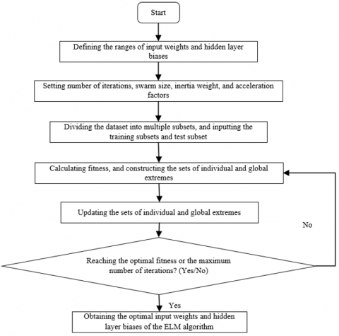
In coalmines, water inrush may be induced by various complex factors. That is why a dozen of secondary indices were selected in our evaluation index system. The more the variables used in prediction, the higher the dimensionality of the ELM parameters. However, the traditional way to explore the correlations between influencing factors, that is, updating ELM parameters through gradient descent, could easily fall into the local minimum trap, and even leads to an incorrect prediction model. Here, the classification performance and running speed are optimized by the PSO algorithm, drawing on the metaheuristic search method. The workflow of the PSO-optimization of the ELM algorithm is explained in Figure 3.
Figure 3. The workflow of the PSO-optimization of the ELM algorithm
Let P=(P1, P2, …, Pn) be a particle swarm in a D-dimensional space, and Pi=(pi1, pi2, …, piD) and Vi=(vi1, vi2, …, viD) be the position and velocity of the i-th particle, respectively. The particles in the swarm iteratively share information with each other, in search of the optimal solution. During the iteration, the i-th particle updates its position and velocity constantly based on the best-known individual position pBest, which is expressed as a matrix Pi=(pi1, pi2, …, piD), and the best-known global position gBest, which is expressed as another matrix Pg=(pg1, pg2, …, pgD):
$V_{id}^{t+1}=\delta V_{id}^{t}+{{a}_{1}}{{\varepsilon }_{1}}\left( P_{id}^{t}-X_{id}^{t} \right)+{{a}_{2}}{{\varepsilon }_{2}}\left( P_{gd}^{t}-X_{id}^{t} \right)$ (5)
$p_{id}^{t+1}=p_{id}^{t}+p_{id}^{t+1}$ (6)
where, d=1, 2, …, D is the dimension of the optimal solution obtained through iterations; t is the number of iterations needed to find the optimal solution; δ is the inertia weight that balances the individual extreme with the global extreme by adjusting the search range; ε1 and ε2 are two random numbers in [0, 1] designed to increase the randomness of the search; a1 and a2 are two acceleration factors that balances the individual extreme with the global extreme by adjusting the number of iterations adaptively in real time. To make the iterative search more pertinent, the particle position and velocity were limited within [-Pmax, Pmax] and [-Vmax, Vmax], respectively. The acceleration factors a1 and a2 can be respectively updated by:
${{a}_{1}}=\left( {{a}_{1h}}-{{a}_{1k}} \right)\frac{t}{{{t}_{\max }}}+{{a}_{1k}}$ (7)
${{a}_{2}}=\left( {{a}_{2h}}-{{a}_{2k}} \right)\frac{t}{{{t}_{\max }}}+{{c}_{2k}}$ (8)
where, a1h, a2h, a1h, and a2h are constants; t is the current number of iterations; tmax is the maximum number of iterations.
During the feature extraction of coalmine water inrush, most evaluation indies can be characterized by Yes or No. The eigenvalues of such indices can be defined as 0 or 1. In this case, the particle velocity can be updated by formula (5), while the particle position can be updated based on the probability that the velocity is mapped to 1 in the interval of [0, 1]. In this way, each evaluation index can be represented by continuous numerical values. Then, corresponding particle velocity can be updated by the sigmoid function:
$\text{sig}V_{id}^{t+1}=\frac{1}{1+{{e}^{-V_{id}^{t+1}}}}$ (9)
The particle position can be updated by:
${{P}_{id}}=\left\{ \begin{align} & 1,if\text{ }\lambda <sig\left( {{V}_{id}} \right) \\ & 0,if\text{ }\lambda \ge sig\left( {{V}_{id}} \right) \\ \end{align} \right.$ (10)
For better computing power and operating efficiency, the ELM algorithm was further improved by the ACO algorithm, which is based on distributed computing. Since the coalmine water inrush prediction involves multiple evaluation indices, the input weights and hidden layer biases were ranked as the nodes of the path traversed by each ant, according to the importance of each evaluation index.
It is assumed that there are R nodes and A ants, and every two adjacent nodes are connected by two paths. Then, an ant faces two path options after arriving at a node: Yes (1) or No (0). Hence, the probability Pi,j for an ant at the i-th node to choose the j-th node can be calculated by:
${{P}_{ij}}=\frac{{{\tau }_{ij}}}{\sum\limits_{i=0}^{R}{{{\tau }_{ij}}}}$ (11)
where, τij pheromone concentration between the i-th node and the j-th node; i=1, 2, …, R; j=0 or 1.
Taking the path of each ant as a feasible solution to coalmine water inrush prediction, the paths of the entire ant colony constitute the solution space of the problem to be optimized. Then, the fitness of the path traversed by an ant, i.e. the absolute error between the ideal output and the real output, can be computed by:
$fitnes{{s}_{ij}}=\frac{1}{R}\sum\limits_{i=1}^{R}{\left| {{I}_{ij}}-{{T}_{ij}} \right|}$ (12)
Then, the obtained solutions are ranked by fitness. The paths corresponding to the optimal solution (optimal paths) are allocated into set O. After that, the path of each ant in the next cycle can be adjusted by formulas (13) and (14), and the pheromone concentration corresponding to the optimal paths, as well as the increment of pheromone concentration, can be updated by the enhancement coefficient ρ:
$\begin{align} & {{\tau }_{ij}}\left( t+1 \right)={{\tau }_{ij}}\left( t \right)+\rho \times \\ & \left[ {\left( fitnes{{s}_{\max }}-fi{{t}_{ij}} \right)}/{\left( fitnes{{s}_{\max }}-fitnes{{s}_{\min }} \right)}\; \right] \\ \end{align}$ (13)
$\Delta {{\tau }_{ij}}=\left\{ \begin{align} & fitnes{{s}_{ij}}/\left( \mu \times A \right),If\text{ }the\text{ }path\in O \\ & 0,\text{ }If\text{ }the\text{ }path\notin O \\ \end{align} \right.$ (14)
where, fitnessmax and fitnessmin are the maximum fitness and minimum fitness, respectively; μ is the proportion of the ants traversing the optimal paths in the colony. The iteration is terminated at the maximum number of iterations tmax, and the maximum fitness in the iteration process can be obtained:
$fitness=\max \left( fitnes{{s}_{t-\max }} \right)$ (15)
where, t=1, 2, …, tmax. The paths corresponding to the maximum paths are recorded to obtain the optimal input weights and hidden layer biases of the ELM algorithm.
So far, this paper relies on combinatory optimization to improve the computing power and operating efficiency of the ELM algorithm. If there are many evaluation indices for coalmine water inrush prediction, there will be a huge number of candidate solutions. In this case, the fitness function should be properly optimized to enhance the generalization ability and classification accuracy of the ELM through training.
To reveal the generalization ability and classification accuracy of each sub-classifier, the original dataset was split into multiple subsets, without changing the properties of the classifier. The last subset was taken as the test subset, and the other subsets as the training subsets. For each subset, the L2-norm of the connection weight β between the hidden layer and the output layer in the ELM network was calculated. Then, the fitness function for the w-th subset can be adjusted into:
$fitnes{{s}_{w}}=\frac{Accurac{{y}_{w}}}{{\overline{\left\| {{\beta }_{w}} \right\|}}/{\overline{\left\| {{\beta }_{all}} \right\|}}\;}$ (16)
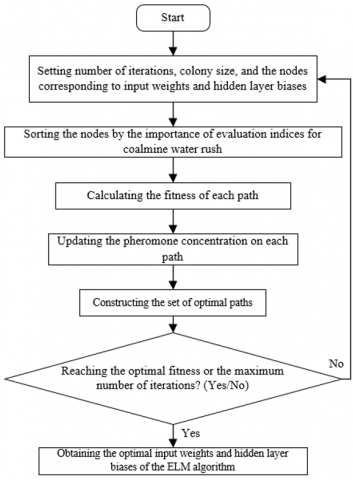
where, Accuracyw is the mean classification accuracy of the w-th subset; the denominator is the mean L2-norm ratio between the weight of each subset and the output weights of all subsets of the ELM network. It can be seen that, with the growing mean classification accuracy of each subset, the L2-norm will decrease, and the fitness will increase. The workflow of the ACO-optimization of the ELM algorithm is explained in Figure 4.
Figure 4. The workflow of the ACO-optimization of the ELM algorithm
In the previous section, the ELM algorithm was subject to combinatory optimization by the PSO and ACO algorithms. The input weights and hidden layer biases of the ELM algorithm were processed in a distributed manner, enhancing the computing power and operating efficiency of the algorithm. Based on the combinatory optimized ELM, a coalmine water inrush prediction model was established in the following steps:
Step 1. The activation function g(x) is determined based on N coalmine water inrush evaluation indices. The ωi and bi are randomly initialized.
Step 2. For the evaluation indices whose values are logical data, the eigenvalues are set to 0 or 1. For those whose values are numerical data, the numerical values are normalized by:
$X_{i}^{\prime}=\frac{X_{i}-X_{i-\min }}{X_{i-\max }-X_{i-\min }}$ (17)
where, x¢i is the normalized value of the inputted evaluation index x¢i; xi-min and xi-max are the minimum and maximum of the i-th evaluation index, respectively.
Step 3. The normalized dataset is decomposed into several subsets, followed by the definition of the training subsets and test subset. Then, the number of iterations, the range of inertia weight, acceleration factors, and random numbers of the PSO algorithm are configured, as well as the termination conditions.
Step 4. A directed node swarm of R nodes is generated, in which each node vector corresponds to a set of input weights and hidden layer biases of the ELM algorithm.
Step 5. Each node is treated as a particle for position and velocity updates, and viewed as a node to be traversed by the ant colony. Then, the nodes are ranked by the importance of evaluation indices.
Step 6. The fitness values of each particle and subset are calculated by the ELM algorithm. On this basis, the set of individual extremes, the set of global extremes, and the set of optimal paths are established for the particle swarm.
Step 7. The fitness values are updated through iterative optimization. Meanwhile, the set of individual extremes, the set of global extremes, and the pheromone concentrations of the ant colony, are all updated.
Step 8. The iterative optimization is terminated if the optimal fitness or the maximum number of iterations is reached. Then, the input weights and hidden layer biases are obtained for the ELM algorithm. Otherwise, Steps 4-8 need to be implemented again.
To reduce the dimension of input samples and improve the training speed of the prediction model, the data on the evaluation indices collected from the coalmine need to be filtered. Therefore, dimensionality reduction was introduced to the subset division process. As shown in Figure 5, the coalmine water inrush prediction with dimensionality reduction can be implemented in the following steps:
Step 1. The evaluation index dataset is numbered, creating 19-dimensional subsets including the original dataset U0: U0, U1, U2, …, U19.
Step 2. The index subsets are imported in turn to the ELM model for training. To analyze the error of the prediction model, the mean error of the ELM model on each test subset is calculated through ten-fold cross-validation. The mean errors corresponding to Ug(g=1, 2, …, 19) are denoted as eg(g=1, 2, …, 19). Comparing e0 with each item in eg(g=1, 2, …, 19), the removal of the corresponding evaluation index does not affect the prediction accuracy of coalmine water inrush, if e0 is the smaller item.
Step 3. Steps 1-2 are repeatedly executed until the number of subsets and mean error on test set are both desirable.
Through the above steps, five indices were removed, including aquifer thickness, coal seam thickness, mining direction, oblique length of working face, and geo-stress. Then, the original dataset was reduced to 14 dimensions. Through dimensionality reduction, the training time of the ELM model was shortened, owing to the decline in the volume of input data, and the training efficiency was effectively improved.
Figure 5. The workflow of coalmine water inrush prediction with dimensionality reduction
To verify its effectiveness, the proposed combinatory optimized ELM prediction model was tested on 150 sets of data collected from the working face in a typical coalmine in Shanxi province, northern China.
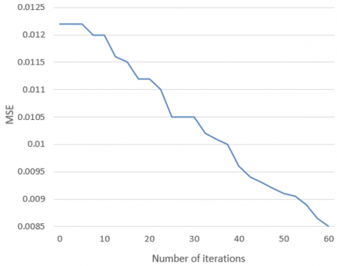
Figure 6. The error change curve of our model
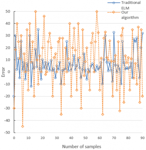
Figure 7. The comparison of prediction errors
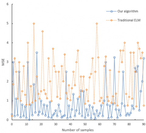
Figure 8. The comparison of MSEs
Figure 6 provides the error change curve of our model. It can be seen that, with the growing number of iterations, the mean squared error (MSE) of our model gradually decreased from 0.01246 to 0.08432.
Figures 7 and 8 compare the errors and MSEs of our algorithm and those of the traditional ELM algorithm in predicting water inrush of the said coalmine. The comparison shows that the mean prediction error and MSE of the traditional ELM algorithm were 15.56 and 2.85, respectively; those of our algorithm were 11.47 and 0.67, respectively. Hence, the proposed algorithm has better prediction accuracy than the traditional ELM algorithm.
Table 1. The comparison of prediction errors and training durations of different algorithms
|
Algorithms |
Mean absolute errors |
MSEs |
Standard deviations |
Mean training durations |
|
BP |
5.1246 |
7.5747 |
8.9362 |
110 |
|
GA-BP |
4.9852 |
6.8747 |
7.7283 |
107 |
|
LSTM |
4.7548 |
6.5797 |
8.7813 |
94 |
|
ELM |
2.7584 |
3.9514 |
4.6326 |
45 |
|
PSO-ELM |
2.4742 |
3.7548 |
3.8547 |
69 |
|
ACO-ELM |
2.7136 |
3.9364 |
4.1567 |
46 |
|
Our algorithm |
1.3649 |
2.2159 |
3.2798 |
71 |
Table 1 compares the prediction errors and training durations of our algorithm with the BP algorithm, the GA-BP algorithm, the long short-term memory (LSTM) algorithm, the traditional ELM algorithm, the PSO-ELM algorithm, and the ACO-ELM algorithm.
It is obvious that our algorithm, as a combinatory optimized algorithm, consumed slightly more time than the traditional ELM algorithm, the PSO-ELM algorithm, and the ACO-ELM algorithm in training, but achieved faster speed than BP, GA-BP, and LSTM algorithms.
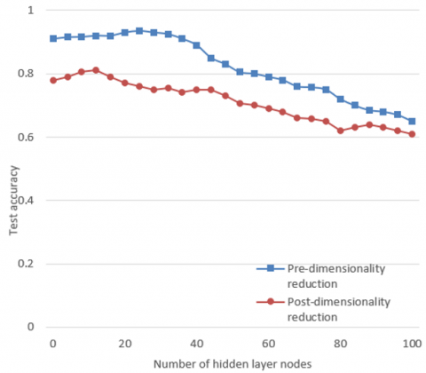
Figure 9 compares the prediction accuracies before and after the dimensionality reduction in subset division. It is clear that the dimensionality reduction improves the prediction effect of our model by removing the redundant evaluation indices for coalmine water inrush.
Figure 9. The comparison of the prediction accuracies before and after the dimensionality reduction
To improve the accuracy, real-time performance and robustness of coalmine water inrush prediction, this paper puts forward an AI-based prediction model for the safety of coalmine water inrush. Firstly, the causes of coalmine water inrush were identified, and used to create a reasonable evaluation index system. Then, the PSO algorithm was combined with the ACO algorithm to optimize the ELM reduction model, and the dimensionality reduction was introduced to subset division. Experimental results show that the proposed combinatory optimized ELM algorithm greatly outperforms other NN algorithms in prediction accuracy and operating speed, and the dimensionality reduction in subset division enhances the prediction effect of our model.
[1] Santana, M.A.D., Pereira, J.M.S., Silva, F.L.D., Lima, N. M.D., Sousa, F.N.D., Arruda, G.M.S.D., Santos, W.P.D. (2018). Breast cancer diagnosis based on mammary thermography and extreme learning machines. Research on Biomedical Engineering, 34(1): 45-53. https://doi.org/10.1590/2446-4740.05217
[2] Mohanty, F., Rup, S., Dash, B., Majhi, B., Swamy, M.N.S. (2019). A computer-aided diagnosis system using Tchebichef features and improved grey wolf optimized extreme learning machine. Applied Intelligence, 49(3): 983-1001. https://doi.org/10.1007/s10489-018-1294-z
[3] Kuppili, V., Biswas, M., Sreekumar, A., Suri, H.S., Saba, L., Edla, D.R., Suri, J.S. (2017). Extreme learning machine framework for risk stratification of fatty liver disease using ultrasound tissue characterization. Journal of Medical Systems, 41(10): 152. https://doi.org/10.1007/s10916-017-0797-1
[4] Preethi, J. (2018). A bio inspired hybrid krill herd-extreme learning machine network based on LBP and GLCM for brain cancer tissue taxonomy. In 2018 3rd International Conference on Computational Intelligence and Applications (ICCIA), pp. 140-144. https://doi.org/10.1109/ICCIA.2018.00033
[5] Gumaei, A., Hassan, M.M., Hassan, M.R., Alelaiwi, A., Fortino, G. (2019). A hybrid feature extraction method with regularized extreme learning machine for brain tumor classification. IEEE Access, 7: 36266-36273. https://doi.org/10.1109/ACCESS.2019.2904145
[6] Pashaei, A., Sajedi, H., Jazayeri, N. (2018). Brain tumor classification via convolutional neural network and extreme learning machines. In 2018 8th International Conference on Computer and Knowledge Engineering (ICCKE), pp. 314-319. https://doi.org/10.1109/ICCKE.2018.8566571
[7] Malik, A., Iqbal, J. (2016). Extreme learning machine based approach for diagnosis and analysis of breast cancer. Journal of the Chinese Institute of Engineers, 39(1): 74-78. https://doi.org/10.1080/02533839.2015.1082934
[8] Toprak, A. (2018). Extreme learning machine (elm)-based classification of benign and malignant cells in breast cancer. Medical Science Monitor: International Medical Journal of Experimental and Clinical Research, 24: 6537. https://doi.org/10.12659/MSM.910520
[9] Salaken, S.M., Khosravi, A., Nguyen, T., Nahavandi, S. (2017). Extreme learning machine based transfer learning algorithms: A survey. Neurocomputing, 267: 516-524. https://doi.org/10.1016/j.neucom.2017.06.037
[10] Xu, Z., Yao, M., Wu, Z., Dai, W. (2016). Incremental regularized extreme learning machine and it׳ s enhancement. Neurocomputing, 174: 134-142. https://doi.org/10.1016/j.neucom.2015.01.097
[11] Geng, Z., Dong, J., Chen, J., Han, Y. (2017). A new self-organizing extreme learning machine soft sensor model and its applications in complicated chemical processes. Engineering Applications of Artificial Intelligence, 62: 38-50. https://doi.org/10.1016/j.engappai.2017.03.011
[12] Chen, C., Jin, X., Jiang, B., Li, L. (2019). Optimizing extreme learning machine via generalized hebbian learning and intrinsic plasticity learning. Neural Processing Letters, 49(3): 1593-1609. https://doi.org/10.1007/s11063-018-9869-6
[13] Zhu, W., Huang, W., Lin, Z., Yang, Y., Huang, S., Zhou, J. (2016). Data and feature mixed ensemble based extreme learning machine for medical object detection and segmentation. Multimedia Tools and Applications, 75(5): 2815-2837. https://doi.org/10.1007%2Fs11042-015-2582-9
[14] Hu, F., Zhou, M., Yan, P., Li, D., Lai, W., Zhu, S., Wang, Y. (2019). Selection of characteristic wavelengths using SPA for laser induced fluorescence spectroscopy of mine water inrush. Spectrochimica Acta Part A: Molecular and Biomolecular Spectroscopy, 219: 367-374. https://doi.org/10.1016/j.saa.2019.04.045
[15] Yang, Y., Yang, J.H., Li, J., Zhang, H.R. (2019). Online discrimination model for mine water inrush source based CNN and fluorescence spectrum. SPECTROSCOPY AND SPECTRAL ANALYSIS, 39(8): 2425-2430.
[16] Han, S., Chen, H., Long, R. (2017). Game analysis of evolution of coal mine safety group behavior based on PT-MA theory. Operations Research and Management.
[17] Winkler, M., Perlman, Y., Westreich, S. (2019). Reporting near-miss safety events: Impacts and decision-making analysis. Safety Science, 117: 365-374. https://doi.org/10.1016/j.ssci.2019.04.029
[18] Kumari, S., Om, H. (2016). Authentication protocol for wireless sensor networks applications like safety monitoring in coal mines. Computer Networks, 104: 137-154. https://doi.org/10.1016/j.comnet.2016.05.007
[19] Henriques, V., Malekian, R. (2016). Mine safety system using wireless sensor network. IEEE Access, 4: 3511-3521. https://doi.org/10.1109/ACCESS.2016.2581844
[20] Zhang, Y., Jing, L., Bai, Q., Liu, T., Feng, Y. (2019). A systems approach to extraordinarily major coal mine accidents in China from 1997 to 2011: An application of the HFACS approach. International Journal of Occupational Safety and Ergonomics, 25(2): 181-193. https://doi.org/10.1080/10803548.2017.1415404
[21] Taylor, P.D., Chen, K., Jonker, L.B., Zhang, M. (2017). Research on coal mine safety supervision mechanism design under managers' overconfidence. Operations Research and Management, 26(11): 182-189.
[22] Ma, Y., Zhao, Q. (2018). Decision-making in safety efforts: Role of the government in reducing the probability of workplace accidents in China. Safety Science, 104: 81-90. https://doi.org/10.1016/j.ssci.2017.12.038
[23] Yu, K., Cao, Q., Xie, C., Qu, N., Zhou, L. (2019). Analysis of intervention strategies for coal miners' unsafe behaviors based on analytic network process and system dynamics. Safety Science, 118: 145-157. https://doi.org/10.1016/j.ssci.2019.05.002
[24] Wu, Y., Chen, M., Wang, K., Fu, G. (2019). A dynamic information platform for underground coal mine safety based on internet of things. Safety Science, 113: 9-18. https://doi.org/10.1016/j.ssci.2018.11.003
[25] Liu, Q., Li, X., Meng, X. (2019). Effectiveness research on the multi-player evolutionary game of coal-mine safety regulation in China based on system dynamics. Safety Science, 111: 224-233. https://doi.org/10.1016/j.ssci.2018.07.014