Yazhou Gao
© 2020 IIETA. This article is published by IIETA and is licensed under the CC BY 4.0 license (http://creativecommons.org/licenses/by/4.0/).
OPEN ACCESS
As the largest manufacturer in the world, China has attracted much attention in the green transformation of manufacturing. This paper firstly designs an evaluation index system (EIS) of green total factor manufacturing energy efficiency (GTFMEE), which covers the three industrial wastes as the undesired output. Based on the EIS, the directional distance function (DDF) was adopted to measure the GTFMEEs of 30 provincial administrative regions (provinces) in China from 2010 to 2017. Then, the Tobit model was introduced to empirically analyze the driving factors of the GTFMEE. The results show that: The different provinces varied significantly in GTFME; the high GTFMEE provinces concentrated in the eastern coastal area, while most inland provinces had undesirable GTFMEEs. The eastern, central, and western regions exhibited different dynamic trends of GTFMEE; the eastern region had much higher GTFMEE than the central and western regions. The GTFMEE has a significant positive correlation with economic growth, technological progress, and opening-up, a significant negative correlation with energy structure, and urbanization level, and an insignificant correlation with human potential.
green total factor manufacturing energy efficiency (GTFMEE), driving factors, directional distance function (DDF), Tobit model
With the rapid advancement of industrialization, China’s manufacturing has mushroomed, and made phenomenal achievements. In terms of manufacturing scale, China surpassed Germany in 2001, overtook Japan in 2007, and replaced the United States (US) 2010 as the largest manufacturer in the world. In 2017, China’s manufacturing achieved an added value of USD 3.55804 trillion, which is 1.64 times that of the US and 27.02% of the global total manufacturing output. Dubbed the world factory, China is now a major manufacturing country, featuring the most complete industrial system and supporting facilities.
The expansion of China’s manufacturing is accompanied by high energy consumption and heavy pollutant emissions. Most manufacturing sectors are energy-intensive. The development of manufacturing inevitably consumes a huge amount of fossil energy. In 2017, China’s manufacturing consumed 2.5090049 billion tons of coal equivalent (TCE), an increase of 3.65 times from that (687.5246 million TCE) in 2000. The high energy consumption leads to heavy emissions of wastewater, waste gas, and solid waste, collectively referred to as the three industrial wastes. In 2017, the industrial sector, which centers on manufacturing, emitted 68.519 trillion standard cubic meters of industrial waste gas, 4.96 times higher than that (13.8145 trillion standard cubic meters) in 2000, and generated 3.31055 billion tons of industrial solid waste, 4.06 times higher than that (816.077 million tons) in 2000.
To sum up, manufacturing brings negative effects like massive energy consumption and serious environmental pollution, while serving as the main driving engine of the economy. To realize sustainable development, China must speed up the energy conservation and emission reduction (ECER), and promote the green transformation and upgrading of manufacturing.
Manufacturing energy efficiency (MEE) has long been a research hotspot. The relevant studies mainly concentrate on four aspects. The first aspect is the evaluation index system (EIS) of MEE. The existing EISs either adopt single-factor index or total-factor index. The typical single-factor index of energy efficiency is the energy consumption per unit output [1, 2]. The total-factor index is the combination of multiple elements, such as capital, labor, and energy [3, 4]. Single-factor index is easy to compute, but fails to consider the issue of factor substitution. Therefore, most scholars prefer to use total-factor index to evaluate the MEE.
The second aspect is the evaluation method of MEE. Data envelopment analysis (DEA) and stochastic frontier analysis (SFA) are the two mainstream methods. Azadeh et al. [5] relied on the DEA model to analyze the energy efficiency of four energy-intensive manufacturing sectors (steelmaking, papermaking, oil refining, and cement production). Lin and Wang [6] used the distance function of the SFA to measure the total factor energy efficiency of China’s steelmaking sector by region, and provided suggestions on energy-saving policies. The SFA requires the establishment of the production function, and only fits for multi-input and single-output problems. The DEA, which is more flexible and adaptive than the SFA, has been adopted by most scholars to measure the MEE.
The third aspect is the evaluation scale of MEE. On the regional level, Miketa and Mulder [7] measured the energy efficiency of 10 manufacturing sectors in 56 developed and developing countries in 1971-1995. On the sector level, papermaking [8], and steelmaking [9] are the common targets in energy efficiency measurement.
The fourth aspect is the factors affecting the MEE. The existing studies have shown that the MEE is greatly affected by enterprise scale [10], technological progress [11], marketization level [12], energy price [13], and government policy [14].
Overall, quite a few results have been achieved on the measurement and influencing factors of the MEE. However, the existing studies have two shortcomings: Many scholars investigated the MEE from the angle of sectors, while few tackled the issue from the angle of regional difference; Most MEE EISs do not contain the various pollutants produced by manufacturing, which inconsistent with the actual situation.
To solve the shortcomings, this paper includes the three industrial wastes into the EIS of green total factor manufacturing energy efficiency (GTFMEE), and adopts the directional distance function (DDF) to measure the GTFMEE of each provincial administrative region (hereinafter referred to as province) in China. Furthermore, the authors examined the driving factors of the GTFMEE. The research results provide an important basis for manufacturers to transform to green development.
2.1 DDF
The MEE measurement has always been a hot topic in the academia. For many years, many scholars measured the MEE solely based on the manufacturing output, without considering the pollutants generated in the manufacturing process. The neglection of environmental cost might cause errors in the measured efficiency [15]. To prevent the error, it is necessary to incorporate the pollutants into the MEE assessment. The MEE that includes environmental factor can be referred to as the GTFMEE.
Since the pollutants are bad outputs, the GTFMEE cannot be effectively measured by traditional tools like Chames-Cooper-Rhodes (CCR) model and Banker-Chames-Cooper (BCC) model, which only apply when all the outputs in the EIS are good. Some scholars tried to evaluate the efficiency after processing these bad outputs. To solve the problem of bad outputs, Hailu and Veeman [16] suggested treating the bad outputs as inputs in efficiency evaluation. This treatment goes against the actual production. Scheel [17] used the reciprocals of the bad outputs in efficiency evaluation. Neither does their strategy work well, for the evaluated efficiency deviates far from the actual efficiency.
The problem of bad outputs was not solved until Chambers et al. [18] proposed the DDF, which perfectly solves the efficiency evaluation involving bad outputs. By the DDF, the bad outputs can be directly incorporated into the EIS as normal outputs, making the evaluation much more accurate. Therefore, the DDF is adopted here to evaluate the GTFMEE. The operation principle of the DDF is as follows:
Let there be a production system of n decision-making units (DMUs), each of which is a complete production process. During the operation, a DMU turns m production factors (inputs) into d units of desired outputs and u units of undesired outputs. For simplicity, the inputs, desired outputs, and undesired outputs are denoted as $X=\left(x_{1}, x_{2}, \ldots, x_{n}\right) \in R_{+}^{m \times n}$ $Y=\left(y_{1}, y_{2}, \ldots, y_{n}\right) \in R_{+}^{d \times n},$ and $b=\left(b_{1}, b_{2}, \ldots, b_{n}\right) \in R_{+}^{u \times n}$ respectively. Let $D M U_{0}=\left(x_{0}, y_{0}^{g}, y_{0}^{b}\right)$ be the DMUs in the production system. Then, the production possibility set (PPS) can be expressed as $P^{t}(x)=\{(x, y): x$ can produce $y\}$. Hence, the DDF can be established as:
$\vec{D}_{0}\left(x, y, b ; g_{y},-g_{b}\right)=\sup _{\theta}\left\{\theta:\left(y+\theta g_{y}, b-g_{b}\right) \in P(x, y, b)\right\}$ (1)
Formula (1) illustrates the operation flow of the entire DDF, i.e. the inputs are converted into desired and undesired outputs. Two basic features of DDF can be observed: (1) Any production activity will lead to undesired outputs b, in addition to desired outputs y; the two kinds of outputs are closely associated with each other. (2) The undesired outputs b are weakly disposable; the reduction of undesired outputs b will definitely cause the desired outputs y to decrease, i.e. the two types of outputs change in the same direction. Drawing on these features, the relative efficiency of each DMU can be solved through linear programming:
$\vec{D}_{0}^{t}\left(x^{t k}, y^{t k}, b^{t k} ; g_{y}^{t k},-g_{b}^{t k}\right)=\max \theta$
s.t. $\sum_{j=1}^{n} \lambda_{j} y_{r j}^{t} \geq(1+\theta) y_{r k}^{t}, r=1,2, \ldots, d$
$\sum_{j=1}^{n} \lambda_{j} b_{l j}^{t}=(1-\theta) b_{l k}^{t}, l=1,2, \ldots, u$
$\sum_{j=1}^{n} \lambda_{j} x_{i j}^{t} \leq(1-\theta) x_{i k}^{t}, i=1,2, \ldots, m$
$\quad \lambda_{j} \geq 0, \quad j=1,2, \ldots, n$ (2)
where, $x^{t k}, y^{t k},$ and $b^{t k}$ are the inputs, desired outputs, and undesired outputs, respectively; $g_{y}^{t k}$ is the increment of desired outputs; $-g_{b}^{t k}$ is the decrement of undesired outputs; θ is the distance between desired outputs and undesired outputs, reflecting the amplitude of the increment of desired outputs and the decrement of undesired outputs. If θ is large, the desired outputs increase significantly, or the undesired outputs decrease significantly; in this case, the DMU has a low efficiency. If θ is small, the desired outputs increase insignificantly, or the undesired outputs decrease insignificantly; in this case, the DMU has a high efficiency. If θ equals 0, both desired and undesired outputs are optimal, leaving no room for improvement; in this case, the DMU efficiency amounts to 1.
2.2 GTFMEE EIS
Our research object, the GTFMEE, is an energy efficiency containing environmental variables. As a total factor, the GTFMEE covers multiple elements, namely, capital, labor, energy, and output [19]. In addition, the GTFMEE was measured from both inputs and outputs. From the angle of inputs, the GTFMEE reflects the ratio of actual energy input to the minimum energy input. The greater the ratio, the larger the gap between actual and minimum energy inputs, and the smaller the GTFMEE. The inverse is also true. From the angle of outputs, the GTFMEE reflects the ratio of actual output to optimal output per unit energy in manufacturing. The greater the ratio, the closer the actual output to the optimal output, and the larger the GTFMEE. The inverse is also true.
Table 1. The GTFMEE EIS
|
Type |
Name |
Meaning |
|
Inputs |
Labor input |
The annual number of urban manufacturing employees in each province (unit: 10,000 persons) |
|
Capital input |
The capital stock in manufacturing is often estimated by permanent inventory method (PIM), which is compute-intensive and error-prone. Considering data availability, the capital input of manufacturing was measured by the total annual investment in fixed assets of manufacturing in each province (unit: RMB 100 million yuan). To eliminate the inflation induced by price factor, the total investment in fixed assets of manufacturing in the current year was converted into the actual total investment in fixed assets of manufacturing at a comparable price with 2010 as the base period, using the price index of investment in fixed assets. |
|
|
Energy input |
The total annual energy consumption of manufacturing in each province (unit: 10,000 TCE). Note that the energy input refers to the terminal consumption, involving such energies as coal, coke, crude oil, diesel, gasoline, natural gas, and electricity. The consumptions of different energies in manufacturing were converted into TCE (unit: 10,000 TCE), and totaled to obtain the energy input. |
|
|
Outputs |
Desired output |
The actual annual total manufacturing output in each province. The statistical yearbooks only provide nominal total manufacturing output. With 2010 as the base period, the nominal total manufacturing output was deflated into the actual total manufacturing output at a comparable price, using the ex-factory price index of industrial products. |
|
Undesired output |
The annual emissions of the three industrial wastes in each province. Due to the difficulty in acquiring the data on the waste gas, wastewater, and solid waste emitted by manufacturing in each province, this paper chooses the three industrial wastes (industrial waste gas emissions, 100 million standard cubic meters; industrial wastewater emissions, 10,000 tons; industrial solid waste emissions, 10,000 tons) as the proxy variable of undesired output. |
Drawing on the concept of GTFMEE and the results of [20, 21], this paper designs a GTFMEE EIS from the angles of inputs and outputs. The designed EIS contains three inputs: labor input, capital input, and energy input of manufacturing. Labor is essential to the production of manufacturers. Without sufficient labor, it is impossible for manufacturers to operate production equipment, or sell their products, not to mention completing the production process. Capital provides a strong support to the production of manufacturers. Sufficient capital guarantees the purchase of production equipment and raw materials, as well as the compensation for labor. Energy is the source of power in the production of manufacturers. Given that most manufacturing sectors are energy-intensive, sufficient energy input is particularly important for manufacturing development.
There are two types of outputs in the designed EIS: Desired output (good output) and undesired output (bad output) of the production of manufacturers. In general, the total output of manufacturing, which reflects the market value of production activities, is the goal pursued by manufacturers. Hence, the total manufacturing output was chosen as the desired output. The undesired output should be avoided in the production process. During the production of manufacturers, the main bad outputs are various pollutants. The most common pollutants are the three industrial wastes. Therefore, the three industrial wastes were collected treated as the undesired output in our EIS.
In summary, our EIS consists of three inputs (labor input, capital input, and energy input), a desired output, and an undesired output. The meaning of each index is explained in Table 1.
2.3 Tobit model
As mentioned before, one of the research objectives is to identify and verify the driving factors of China’s GTFMEE, laying the basis for formulating scientific ECER policies. To verify every factor that drives the GTFMEE, it is critical to select a suitable measurement model.
According to the above definition of the GTFMEE, the efficiency calculated by the DDF is limited between 0 and 1. As the dependent variable in the measurement model, the GTFMEE must fall within the interval of [0, 1], that is, the upper and lower limits of the variable are 0 and 1, respectively. If the traditional ordinary least squares (OLS) is adopted for model estimation, the results might be biased toward zero, and the model estimation will be distorted [22].
The Tobit model, named after its proposer, can effectively prevent the data truncation of the dependent variable. Also known as truncated or censored regression model, the Tobit model only works when the dependent variable has a limited range. This unique property adapts well to the needs of significance test on GTFMEE driving factors.
Before establishing the Tobit model, it is necessary to identify the driving factors of the GTFMEE. The previous research has demonstrated that the MEE could be greatly impacted by economic growth, technological progress, opening-up, and energy structure [23, 24].
Inspired by the previous research, the driving factors of the GTFMEE were summarized as physical factors, affair factors, and human factors. Specifically, the physical factors include economic growth (EG), and technological progress (TP); the affair factors include opening-up (OU), and energy structure (ES); the human factors include human potential (HP), and urbanization level (UL). Taking the GTFMEE as the dependent variable, and the driving factors as the independent variables, the following Tobit model can be established:
$M I G T F E E_{i t}^{*}=\alpha+\beta_{1} E G_{i t}+\beta_{2} T P_{i t}+\beta_{3} O U_{i t}+\beta_{4} E S_{i t}+\beta_{5} H P_{i t}+\beta_{6} U L_{i t}+\varepsilon$
$\left\{\begin{array}{l}M I G T F E E_{i t}=M I G T F E E_{i t}^{*}\left(\text {if } M I G T F E E_{i t}^{*}<1\right) \\ M I G T F E E_{i t}=1 \quad\left(\text {if } M I G T F E E_{i t}^{*} \geq 1\right)\end{array}\right.$ (3)
where, MIGTFEEit is the dependent variable; EGit is economic growth (the per-capita gross domestic product (GDP) of province i in year t);TPit is technological progress (the internal expenditure on research and development (R&D) of industrial enterprises as a proportion of industrial added value of province i in year t); OUit is opening-up (the actual foreign direct investment (FDI) in RMB as a proportion of GDP of province i in year t); ESit is energy structure (the coal consumption as a proportion of total energy consumption of province i in year t); HPit is human potential (mean education years of labor force of province i in year t); ULit is urbanization level (permanent urban population as a proportion of the total population of province i in year t).
Note that: (1) the natural logarithm of economic growth was adopted to eliminate the impact of potential collinearity; (2) the technological progress was replaced by the internal expenditure on R&D of industrial enterprises as a proportion of industrial added value, because most industrial enterprises in China are manufacturers, and the internal R&D expenditure in manufacturing is unavailable; (3) the mean education years of labor force was calculated by:
The mean education years of labor force = the proportion of employees in the illiterate and semi-illiterate * 1.5 + the proportion of employees in primary school graduates *7.5 + the proportion of employees in junior high school graduates *10.5 + the proportion of employees in senior high school graduates * 13.5 + the proportion of employees in graduates from junior college and above *17.
2.4 Data sources
To ensure the availability and comparability of each variable in the DDF and Tobit model, this paper selects the panel data on 30 Chinese provinces in 2010-2017 as the samples (excluding Tibet, Hong Kong, Macao, and Taiwan). The data on the number of urban manufacturing employees, the total investment in fixed assets of manufacturing, the price index of investment in fixed assets, the total energy consumption of manufacturing, the total manufacturing output, the industrial waste gas emissions, the industrial wastewater emissions, the industrial solid waste emissions, the internal expenditure on R&D of industrial enterprises, the industrial added value, the actual FDI, GDP, coal consumption, total energy consumption, the proportions of employees in the population with different education backgrounds, the permanent urban population, and the total population were obtained from China Statistical Yearbooks, China Energy Statistical Yearbooks, China Labor Statistical Yearbooks, China Statistical Yearbooks on Environment, China Statistical Yearbooks on Science and Technology, China Industry Statistical Yearbooks, local statistical yearbooks, and the official website of National Bureau of Statistics of China. The few missing data were completed by moving average method.
3.1 Measuring results on GTFMEE
The data on the inputs and outputs in our GTFMEE IES were imported into maxDEA, and the DDF was adopted to measure the GTFMEEs of the 30 Chinese provinces in 2010-2017. The measured results are recorded in Table 2.
As shown in Table 2, the GTFMEEs in China differed greatly from province to province. In the sample period, Beijing, Tianjin, Hebei, and Shanghai were the only provinces whose GTFMEE remained at the optimal value of 1. The GTFMEEs of these provinces fell on the efficient frontier for the following reasons: Beijing, Tianjin, and Shanghai, as municipalities directly under the central government, boast developed economy and advanced manufacturing technology, and attach great importance to the ECER. Located in the eastern coastal area, Hebei is adjacent to Beijing and Tianjin. Its GTFMEE is optimized by its advantageous location advantage and early start in manufacturing.
The mean GTFMEEs of Guangdong, Shandong, Jiangsu, Zhejiang, and Hubei fell between 0.9 and 1. The GTFMEEs of these provinces reached 1 in some years, and fell short of 1 in the other years, leaving a room for improvement. Except Hubei, Guangdong, Shandong, Jiangsu, and Zhejiang are eastern coastal provinces with large manufacturing scale and high manufacturing output. However, the manufacturers in these provinces emit many pollutants, especially the three industrial wastes, in the production process. These provinces must step up the efforts in ECER. Note that Hubei achieved desirable GTFMEE, despite being a central province. The achievement is inseparable from the green transformation of manufacturing in that province.
The mean GTFMEEs of Anhui, Jilin, Liaoning, Inner Mongolia, Hainan, Hunan, Fujian, Jiangxi, Henan, Chongqing, and Sichuan ranged from 0.7 to 0.9. The GTFMEEs of these provinces belong to the mid-level in China, with a certain distance from the efficient frontier. Further improvement is needed in the future. In recent years, these provinces have witnessed rapid industrial development, and continuous expansion of manufacturing. But their GTFMEEs are not desirable, because the local manufacturers develop extensively, consume lots of energy, use energy non-intensively, and overlook pollution control.
The mean GTFMEEs of Guangxi, Ningxia, Gansu, Xinjiang, Shaanxi, Guizhou, Yunnan, Heilongjiang, Shanxi, and Qinghai were below 0.7, falling behind those of most other provinces. The GTFMEEs in these provinces are extremely unsatisfactory, waiting to be substantially improved. As late starters in industry, these inland provinces are relatively backward in terms of economy. In particular, the local manufacturers are small, lacking advanced production technology. These factors, coupled with the inefficient energy use, lead to heavy pollutant emissions. As a result, these provinces are slow in the green transformation of manufacturing.
To sum up, the different provinces varied significantly in GTFMEE. The high GTFMEE provinces concentrated in the eastern coastal area, while most inland provinces had undesirable GTFMEEs. Hence, the development of manufacturing in China shows obvious regional imbalance. To grow into a strong manufacturer, China must mitigate the regional imbalance of manufacturing development.
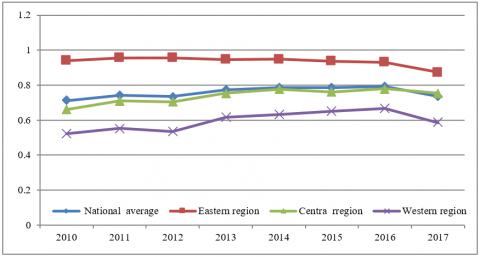
Geographically, China can be divided into eastern region, central region, and western region. To further examine the regional difference in GTFMEE, the change trends of GTFMEE in China and the three regions are plotted as Figure 1.
It can be seen that the GTFMEE of the central region changed similarly as the national GTFMEE: both slowly increased in the sample period. The GTFMEE of the eastern region remained relatively stable, with insignificant change in the early phase and slight decline in the late phase. The GTFMEE of the western region exhibited an inverted U-shaped trend, i.e. first increased and then decreased.
Table 2. The GTFMEEs of Chinese provinces in 2010-2017
|
Province |
2010 |
2011 |
2012 |
2013 |
2014 |
2015 |
2016 |
2017 |
Mean |
|
Beijing |
1.0000 |
1.0000 |
1.0000 |
1.0000 |
1.0000 |
1.0000 |
1.0000 |
1.0000 |
1.0000 |
|
Tianjin |
1.0000 |
1.0000 |
1.0000 |
1.0000 |
1.0000 |
1.0000 |
1.0000 |
1.0000 |
1.0000 |
|
Hebei |
1.0000 |
1.0000 |
1.0000 |
1.0000 |
1.0000 |
1.0000 |
1.0000 |
1.0000 |
1.0000 |
|
Shanghai |
1.0000 |
1.0000 |
1.0000 |
1.0000 |
1.0000 |
1.0000 |
1.0000 |
1.0000 |
1.0000 |
|
Guangdong |
1.0000 |
1.0000 |
1.0000 |
1.0000 |
1.0000 |
1.0000 |
0.9766 |
0.8675 |
0.9805 |
|
Shandong |
0.9126 |
1.0000 |
1.0000 |
1.0000 |
1.0000 |
1.0000 |
1.0000 |
0.8637 |
0.9720 |
|
Jiangsu |
1.0000 |
1.0000 |
1.0000 |
1.0000 |
1.0000 |
0.9354 |
0.9256 |
0.8451 |
0.9633 |
|
Zhejiang |
1.0000 |
1.0000 |
1.0000 |
1.0000 |
1.0000 |
0.9694 |
0.9121 |
0.8038 |
0.9607 |
|
Hubei |
0.8172 |
0.8811 |
0.9427 |
0.9513 |
0.9587 |
0.9394 |
0.9556 |
0.8723 |
0.9148 |
|
Anhui |
0.8076 |
0.8808 |
0.8341 |
0.8678 |
0.8786 |
0.9156 |
0.9358 |
0.8873 |
0.8759 |
|
Jilin |
0.7818 |
0.8311 |
0.8371 |
0.9022 |
1.0000 |
0.8826 |
0.8694 |
0.8600 |
0.8705 |
|
Liaoning |
0.9826 |
0.9177 |
0.9494 |
1.0000 |
0.8793 |
0.6647 |
0.6776 |
0.6667 |
0.8423 |
|
Inner Mongolia |
0.8510 |
0.8695 |
0.7276 |
0.9200 |
0.8120 |
0.7491 |
0.7679 |
0.7925 |
0.8112 |
|
Hainan |
0.7157 |
0.7769 |
0.7751 |
0.6177 |
0.8031 |
0.9373 |
0.9493 |
0.7985 |
0.7967 |
|
Hunan |
0.6336 |
0.7095 |
0.6433 |
0.7968 |
0.8516 |
0.8639 |
0.9510 |
0.9007 |
0.7938 |
|
Fujian |
0.7153 |
0.8039 |
0.8006 |
0.7888 |
0.7500 |
0.7832 |
0.7871 |
0.7518 |
0.7726 |
|
Jiangxi |
0.7396 |
0.7315 |
0.7501 |
0.7934 |
0.8162 |
0.7758 |
0.7615 |
0.6608 |
0.7536 |
|
Henan |
0.7023 |
0.7353 |
0.7563 |
0.7464 |
0.7542 |
0.7206 |
0.7825 |
0.7820 |
0.7474 |
|
Chongqing |
0.6589 |
0.7136 |
0.7098 |
0.7812 |
0.8334 |
0.8058 |
0.8435 |
0.6132 |
0.7449 |
|
Sichuan |
0.6384 |
0.6999 |
0.6623 |
0.6381 |
0.7423 |
0.7862 |
0.7898 |
0.6701 |
0.7034 |
|
Guangxi |
0.5335 |
0.5881 |
0.5659 |
0.6987 |
0.7274 |
0.7617 |
0.8171 |
0.8568 |
0.6936 |
|
Ningxia |
0.4883 |
0.4879 |
0.5486 |
0.6754 |
0.6134 |
0.6226 |
0.6679 |
0.5769 |
0.5851 |
|
Gansu |
0.4956 |
0.5646 |
0.5513 |
0.5858 |
0.5886 |
0.6146 |
0.5573 |
0.5927 |
0.5688 |
|
Xinjiang |
0.5769 |
0.4563 |
0.4522 |
0.5810 |
0.5336 |
0.5473 |
0.5783 |
0.5297 |
0.5319 |
|
Shaanxi |
0.4134 |
0.4747 |
0.4927 |
0.4868 |
0.5119 |
0.5529 |
0.5757 |
0.4393 |
0.4934 |
|
Guizhou |
0.3203 |
0.3840 |
0.3470 |
0.4578 |
0.5504 |
0.6742 |
0.6570 |
0.5139 |
0.4881 |
|
Yunnan |
0.4045 |
0.4668 |
0.4836 |
0.4979 |
0.5129 |
0.5189 |
0.5036 |
0.4534 |
0.4802 |
|
Heilongjiang |
0.3973 |
0.4125 |
0.4074 |
0.5079 |
0.4889 |
0.5258 |
0.5284 |
0.5443 |
0.4765 |
|
Shanxi |
0.4162 |
0.5030 |
0.4592 |
0.4617 |
0.4696 |
0.4565 |
0.4521 |
0.5359 |
0.4693 |
|
Qinghai |
0.3548 |
0.3699 |
0.3576 |
0.4694 |
0.5144 |
0.5287 |
0.5793 |
0.4106 |
0.4481 |
In addition, the three regions had marked differences in mean GTFMEE. In the sample period, the mean GTFMEE of the eastern region was as high as 0.9353, far exceeding the national average of 0.7980. The mean GTFMEE of the central region was 0.7377, comparable to the national average. The mean GTFMEE of the western region was 0.5953, far below the national average. Thus, the eastern region had the highest GTFMEE, followed in turn by the central region, and the western region. Obviously, the central and western regions are the weak links of China’s manufacturing development.
Figure 1. The change trends of GTFMEE in China and the three regions
3.2 Results analysis of Tobit model
Based on the proposed Tobit model, the significance of each driving factor of GTFMEE was tested on Stata12.0. The estimated results on the coefficients of the independent variables are recorded in Table 3.
Table 3. The regression results of Tobit model
|
Variable |
Coefficient |
T-value |
P-value |
|
EG |
0.2738*** |
4.47 |
0.000 |
|
TP |
4.6408*** |
3.55 |
0.000 |
|
OU |
4.1730*** |
5.14 |
0.000 |
|
ES |
-0.1342*** |
-3.34 |
0.001 |
|
HP |
0.0326 |
1.31 |
0.192 |
|
UL |
-0.4876* |
-1.73 |
0.085 |
|
L- likelihood |
46.4345 |
||
Note: *, **, and *** are the significance levels of 10%, 5%, and 1%, respectively.
The influence of economic growth (EG) on the GTFMEE was positive at the significance level of 1%, indicating that higher per-capita GDP promotes the GTFMEE. It can also be seen that the level of economic development provides manufacturing development with the necessary capital and high-quality labor force, which in turn promote the structural optimization and upgrading of manufacturing. This benefits the green transformation of manufacturers.
The estimated coefficient of technological progress (TP) was positive, passing the significance test at 1%. Hence, the growing R&D expenditure promotes the GTFMEE. It can be said that, two benefits will be generated, when the industry, represented by manufacturing, invests more in R&D: On the one hand, the manufacturers will be blessed with advanced technology, which improves the efficiency of energy use; on the other hand, advanced technologies, such as cloud computing, three-dimensional (3D) printing, and industrial intelligence, fuel the upgrading of manufacturing from low end to high end, and enhance the market competitiveness of manufacturers. Fisher-Vanden et al. [25] investigated the micro-data of large and medium-sized Chinese manufacturers, and found that technological progress is the main reducer for energy intensity of manufacturing: R&D investment contributes to 12% of energy efficiency.
Opening-up (OU) exerted a significantly positive impact on the GTFMEE, indicating that a high proportion of FDI in GDP boosts the GTFMEE. Opening-up is the fundamental strategy of China in the long term. For a long time, the Chinese government has been vigorously attracting foreign investment: diverting foreign funds to develop manufacturing, and absorbing production technology and management experience of foreign-funded enterprises. Erdem [26] also confirmed that the technology diffusion effect of FDI can improve the energy efficiency of enterprises in host country.
Energy structure (ES) had a significant negative effect on the GTFMEE, that is, a high proportion of coal consumption in the total region energy consumption hinders the improvement of the GTFMEE. Coal has long been considered as the most unclean energy source. The combustion of coal releases multiple harmful pollutants. As a major coal producer and consumer, China has difficulty in the ECER of manufacturing, facing the coal-dominated energy structure. Shi et al. [27] evaluated the highest energy efficiency and energy-saving potential of various provinces in China, revealing that coal-rich provinces generally have low energy efficiency.
Human potential (HP) had an insignificant positive impact on the GTFMEE. This means improving the education level of the labor force can help increase personal labor productivity and enhance environmental awareness, exerting a positive impact on the ECER of manufacturers. However, only a few Chinese provinces have an abundance of high-end manufacturing talents. These talents are severely lacking in most provinces. According to the data of 58.com, a famous classified advertisements website, the labor gaps of manufacturing in Beijing and Shanghai reached 52% and 44% in 2016, respectively. Suffice it to say that labor shortage is commonplace in China’s manufacturing. In short, the insignificant impact of human potential on the GTFMEE comes from the severe shortage of high-quality labor force.
The impact of urbanization level (UL) on the GTFMEE was positive at the 1% significance level, meaning that higher urbanization level inhibits the green transformation of manufacturing. A possible reason lies in the extensive model of urbanization in China. Over the years, urban construction in China emphasizes quantity over quality. In the early phase of urbanization, low-end manufacturing sectors with high energy consumption are welcomed, due to their low threshold and investment. As a result, the energy consumption of manufacturing remains high, bringing heavy pollutant emissions.
This paper sets up a DDF containing undesired outputs, and applies it to measure the GTFMEEs of 30 Chinese provinces in 2010-2017. In addition, the Tobit model was adopted to verify the driving factors of the GTFMEE. The main conclusions are as follows:
First, the GTFMEEs in China differed greatly from province to province in the sample period. Specifically, Beijing, Tianjin, Hebei, and Shanghai achieved the optimal GTFMEE, which reached the efficient frontier; the GTFMEEs of Guangdong, Shandong, Jiangsu, Zhejiang, and Hubei were relatively desirable, leaving a room for improvement. The GTFMEEs of Anhui, Jilin, Liaoning, Inner Mongolia, Hainan, Hunan, Fujian, Jiangxi, Henan, Chongqing, and Sichuan belong to the mid-level in China, requiring further improvement in the future. The GTFMEEs of Guangxi, Ningxia, Gansu, Xinjiang, Shaanxi, Guizhou, Yunnan, Heilongjiang, Shanxi, and Qinghai were extremely unsatisfactory, waiting to be substantially improved.
Second, the eastern, central, and western regions had marked differences in GTFMEE. The three regions exhibited different dynamic trends of GTFMEE. The eastern region had the highest GTFMEE, followed in turn by the central region, and the western region.
Third, among the driving factors, economic growth, technological progress, and opening-up had significant positive impact on the GTFMEE; energy structure, and urbanization level had significant negative impact on the GTFMEE; human potential exerted an insignificant impact on the GTFMEE.
[1] Patterson, M.G. (1996). What is energy efficiency?: Concepts, indicators and methodological issues. Energy Policy, 24(5): 377-390. https://doi.org/10.1016/0301-4215(96)00017-1
[2] Alcantara, V., Duarte, R. (2004). Comparison of energy intensities in European Union countries. Results of a structural decomposition analysis. Energy Policy, 32(2): 177-189. https://doi.org/10.1016/S0301-4215(02)00263-X
[3] Mandil, C. (2007). Tracking industrial energy efficiency and CO2 emissions. Paris, International Energy Agency.
[4] Honma, S., Hu, J.L. (2014). Industry-level total-factor energy efficiency in developed countries: A Japan-centered analysis. Applied Energy, 119(10): 67-78. https://doi.org/10.1016/j.apenergy.2013.12.049
[5] Azadeh, A., Amalnick, M. S., Ghaderi, S.F., Asadzadeh, S.M. (2007). An integrated DEA PCA numerical taxonomy approach for energy efficiency assessment and consumption optimization in energy intensive manufacturing sectors. Energy Policy, 35(7): 3792-3806. https://doi.org/10.1016/j.enpol.2007.01.018
[6] Lin, B.Q., Wang, X.L. (2014). Exploring energy efficiency in China׳ s iron and steel industry: A stochastic frontier approach. Energy Policy, 72: 87-96. https://doi.org/10.1016/j.enpol.2014.04.043
[7] Miketa, A., Mulder, P. (2005). Energy productivity across developed and developing countries in 10 manufacturing sectors: Patterns of growth and convergence. Energy Economics, 27(3): 429-453. https://doi.org/10.1016/j.eneco.2005.01.004
[8] Zheng, Q., Lin, B. (2017). Industrial polices and improved energy efficiency in China’s paper industry. Journal of Cleaner Production, 161: 200-210. https://doi.org/10.1016/j.jclepro.2017.05.025
[9] Worrell, E., Price, L., Martin, N. (2001). Energy efficiency and carbon dioxide emissions reduction opportunities in the US iron and steel sector. Energy, 26(5): 513-536. https://doi.org/10.1016/S0360-5442(01)00017-2
[10] Subrahmanya, M.H.B. (2006). Labour productivity, energy intensity and economic performance in small enterprises: A study of brick enterprises cluster in India. Energy Conversion and Management, 47(6): 763-777. https://doi.org/10.1016/j.enconman.2005.05.021
[11] Wei, Y.M., Liao, H., Fan, Y. (2007). An empirical analysis of energy efficiency in China's iron and steel sector. Energy, 32(12): 2262-2270. https://doi.org/10.1016/j.energy.2007.07.007
[12] Kim, J.W., Lee, J.Y., Kim, J.Y., Lee, H.K. (2006). Sources of productive efficiency: International comparison of iron and steel firms. Resources Policy, 31(4): 239-246. https://doi.org/10.1016/j.resourpol.2007.03.003
[13] Birol, F., Keppler, J.H. (2000). Prices, technology development and the rebound effect. Energy Policy, 28(6-7): 457-469. https://doi.org/10.1016/S0301-4215(00)00020-3
[14] Flues, F., Rübbelke, D., Vögele, S. (2015). An analysis of the economic determinants of energy efficiency in the European iron and steel industry. Journal of Cleaner Production, 104: 250-263. https://doi.org/10.1016/j.jclepro.2015.05.030
[15] Nanere, M., Fraser, I., Quazi, A., D’Souza, C. (2007). Environmentally adjusted productivity measurement: An Australian case study. Journal of Environmental Management, 85(2): 350-362. https://doi.org/10.1016/j.jenvman.2006.10.004
[16] Hailu, A., Veeman, T.S. (2001). Non-parametric productivity analysis with undesirable outputs: an application to the Canadian pulp and paper industry. American Journal of Agricultural Economics, 83(3): 605-616. https://doi.org/10.1111/0002-9092.00181
[17] Scheel, H. (2001). Undesirable outputs in efficiency valuations. European Journal of Operational Research, 132(2): 400-410. https://doi.org/10.1016/S0377-2217(00)00160-0
[18] Chambers, R.G., Chung, Y., Färe, R. (1996). Benefit and distance functions. Journal of Economic Theory, 70(2): 407-419. https://doi.org/10.1006/jeth.1996.0096
[19] Hu, J.L., Wang, S.C. (2006). Total-factor energy efficiency of regions in China. Energy Policy, 34(17): 3206-3217. https://doi.org/10.1016/j.enpol.2005.06.015
[20] Mukherjee, K. (2008). Energy use efficiency in US manufacturing: A nonparametric analysis. Energy Economics, 30(1): 76-96. https://doi.org/10.1016/j.eneco.2006.11.004
[21] Long, X., Zhao, X., Cheng, F. (2015). The comparison analysis of total factor productivity and eco-efficiency in China's cement manufactures. Energy Policy, 81: 61-66. https://doi.org/10.1016/j.enpol.2015.02.012
[22] Griliches, Z. (1986). Productivity R & D and basic research at firm level in the 1970’s. American Economic Review, 76(1):141-153.
[23] Zhao, X.L., Yang, R., Ma, Q. (2014). China's total factor energy efficiency of provincial industrial sectors. Energy, 65: 52-61. https://doi.org/10.1016/j.energy.2013.12.023
[24] Imbruno, M., Ketterer, T.D. (2018). Energy efficiency gains from importing intermediate inputs: Firm-level evidence from Indonesia. Journal of Development Economics, 135: 117-141. https://doi.org/10.1016/j.jdeveco.2018.06.014
[25] Fisher-Vanden, K., Jefferson, G.H., Liu, H., Tao, Q. (2004). What is driving China’s decline in energy intensity? Resource and Energy Economics, 26(1): 77-97. https://doi.org/10.1016/j.reseneeco.2003.07.002
[26] Erdem, D. (2012). Foreign direct investments, energy efficiency, and innovation dynamics. Mineral Economics, 24(2-3): 119-133. https://doi.org/10.1007/s13563-012-0015-z
[27] Shi, G.M., Bi, J., Wang, J.N. (2010). Chinese regional industrial energy efficiency evaluation based on a DEA model of fixing non-energy inputs. Energy Policy, 38(10): 6172-6179. https://doi.org/10.1016/j.enpol.2010.06.003