Alireza Hajipour | Arash Mirabdolah Lavasani* | Mohammad Eftekhari Yazdi
© 2021 IIETA. This article is published by IIETA and is licensed under the CC BY 4.0 license (http://creativecommons.org/licenses/by/4.0/).
OPEN ACCESS
Modelling of turbulence is a vital issue for flow forecasting which is of great interest for most of engineering applications like flow over planes, movement of pollutants and some industrial processes. Originally, via solving the government equations (Navier-Stokes equations) the flow field can be simulated. With developing PCs and high-performance computers, implementing of Navier-Stokes equations for numerical simulation is increasing. In this research, the effects of some wall functions on aerodynamic and turbulence behavior of air flow around a simplified high-speed train via OpenFOAM software are numerically investigated. In the following, first, the effects of some default and common wall functions of OpenFOAM on the flow and aerodynamic key parameters are analyzed and then, a relatively new wall function called “Enhanced Wall Function” was implemented from ANSYS FLUENT into OpenFOAM and improvement for comprehensive simulation. Variations of flow key parameters such as velocity, pressure distribution and aerodynamic significant components and parameters such as lift, drag and side coefficients under the influence of wall functions changes are illustrated. The results could be used for obtaining more accurate analysis of aerodynamic characteristics of fluid flow around high-speed trains.
computational fluid dynamics, high-speed train, wall function, aerodynamics, turbulence
In engineering and natural science applications, flow and movement are profoundly influenced by the turbulence phenomena. Compared with the laminar flow, turbulent flow simulation needs advanced numerical methods. Even for small issues, we are forced to do complex computations. Also, fluid flow is limited by walls evermore, so the previous equations and methods are not executable near the wall. Flow behavior near the wall is a complex phenomenon; for this purpose, the different function was investigated. So, a non-dimensional quantity that determines the measured distance from the wall in the viscous area can be considered. One important problem in computational fluid dynamics (CFD) is how to simulate near wall conditions and sublayers where the viscosity impact will be significant. Using a suitable grid and low-Reynolds number method is the confident approach to the solution, but this way is very expensive for three-dimensional problems. Second problem is the very slow convergence especially in the small grids (see Figure 1).
From a physical point of view; near wall region modelling is significant, insomuch solid walls are the basic factor of turbulence and vorticity (local extreme of turbulent kinetic energy and great varieties of turbulence dissipation) and in engineering usages; wall main parameters (pressure, velocity gradients, etc.) are so significant in different applications and also, flow separation are forcefully dependent on an accurate prediction of the development of turbulence near walls.
Considering a solid wall and its effect is very effective in the study of fluid flow and its turbulence. Patankar et al. [1] in 1970, developed “wall function”, a new method, to simplify and find the exact solution of the problems. They argued that the structure of the boundary layer equations, for example wall law, can be accompanied by numerical methods; as a result, there is no need to solve boundary layer equations in turbulence regions.
Figure 1. Wall function approach (first grid point in log-law region: $\left(50 \leq y^{+} \ll 500\right)$, Two-Layer zonal model approach (First grid point at: $y^{+} \approx 1$)
Wall functions are a series of semi-experimental relations which, in effect, “link” or “bridge” the solution parameters close to wall and its related parameters on it. The wall functions included:
• Laws of the wall for temperature and mean velocity (or other quantities).
• Relationships for close to wall turbulent values.
Based on this approach, the characteristic velocity of flow near wall region, can defined as:
$u^{*}=\sqrt{\frac{\tau_{w}}{\rho_{w}}}$ (1)
where, τw and ρw are shear stress and density of wall, respectively. Using the above equation, the non-dimensional velocity, and the non-dimensional length, y+ are defined as follows:
$u^{+}=\frac{u}{u^{*}}$ (2)
and
$y^{+}=\frac{u^{*} \times y}{v}$ (3)
where, $u, y,$ and $v$ are parallel velocity of wall, distance to wall and kinematic viscosity, respectively. Moreover, turbulent flows are divided into the inner and outer layers; in the inner layer there are three flow regions as follows:
The log-law region with fully turbulent flow $\left(u^{+}=\frac{1}{k} \operatorname{Ln}\left[y^{+}\right]+B\right)$.
Generally, the equations which describe the velocity profile in inner region are called “law of the wall”.
In recent years, many simulations of flow over high-speed trains have been performed. The most significand and related of them reviewed by Rashidi et al. in 2019 [2] which are listed as follow:
In 2002, an experimental and numerical investigation of air flow around a high-speed train was done by Paradot et al. [3]. In this research, a high-speed train at French railways among a turbulent air flow was simulated, numerically using the commercial code Star CD. Khier et al. [4] in 2002 performed side wind influence on a German InterRegio high-speed train by a numerical simulation using RANS and k-ε turbulence approach. In this simulation, the aerodynamic forces and the flow structure under the yaw angles change were investigated. In 2002, Fauchier et al. [5] simulated the influences of crosswind on InterRegio high-speed train, a German train, using RANS approach. To achieve this, a simple geometry train model was considered and a CFD analysis and second an aerodynamic investigation on the train were performed. An aerodynamic simulation of flow behavior on a high-speed train was investigated by Shin et al. in 2003 [6]. In this simulation, the aerodynamic forces were calculated at the entrance of the tunnel. Thus, the vortex and pressure structures of the air turbulent flow around the high-speed train were illustrated. Tian [7] investigated an aerodynamic simulation on a high-speed train in 2009. In this research, the drag aerodynamic force as an effective factor in energy consumption and the shape and geometry of the train nose were discussed and using the bottom cover and outer wind shields was suggested to reduce aerodynamic forces. In 2009, Zhao et al. [8] performed an aerodynamic property of a Chinese high-speed train via RANS numerical approach. To achieve this, two sizes of tunnel and four various velocity of the train as 200, 250, 300 and 350 km/h were considered. the aerodynamic forces and pressure distribution and their effects on the train body especially at the entrance and exit of the tunnel were the most significant results of the article. In 2009, an aerodynamic simulation of a high-speed train using RANS numerical approach was done by Krajnović [9]. Also, a genetic algorithm was applied to optimize the aerodynamic behavior of a Swedish high-speed train. Drag reduction and vortex produced for crosswind stability were the principal goals of the optimization. Li et al. [10] did a RANS numerical simulation on a simple model of electric multiple units (EMU) at a tunnel entrance in 2011. The influences of the microwaves and the wall pressure range of the tunnel on aerodynamic behavior of the air flow around the train were investigated. In 2012, a RANS numerical simulation of an EMU high-speed train was investigated by Wang et al. [11]. In this research, for two trains passing alongside each other in a tunnel, the aerodynamic forces and pressure changes were analyzed. A similar analysis was conducted for passing an EMU high-speed train through the tunnel. A simulation of flow over a simplified train model via Partially averaged Navier Stokes was conducted by Östh et al. [12] in 2012. Two cases in this research were considered, the first case was natural flow over the high-speed train and the second one was a cavity was placed on the base of the train. For these two cases, the aerodynamic drag force and the pressure coefficient were calculated and compared. Moreover, a comparison between the CFD findings and related experimental data was done. In 2014, Asress et al. [13] did a URANS numerical investigation of a high-speed train against a crosswind. They considered two different scenarios for the ground, the first was static ground and the second was moving one. Then the streamlines, the flow structure and velocity contour for different yaw angles as 30° to 60° were simulated. Peng et al. [14] in 2014, performed a RANS numerical approach simulation for wind influence on a high-speed train. In this paper, two cases of aerodynamic simulation were considered. The first case was a train passing through the tunnel and the second one was two trains passing through the tunnel side by side. In 2014, Shuanbao et al. [15] did an optimization of aerodynamic parameters for CRH380A high-speed trains using RANS numerical approach. At the first, the aerodynamic forces were analyzed and then, a multi-objective optimization using a genetic algorithm (GA) method was performed. Finally, an aerodynamic comparison between the optimal shape of the train with the original one was presented. A RANS numerical approach for simulation of two high-speed trains in a tunnel was done by Chu et al. [16] in 2014. The main goal of this research was pressure wave analysis. Also, effects of some significant parameters as the train length and velocity on the aerodynamic waves generated by the train were performed. In the following it was determined that the pressure and aerodynamic drag in which area reach the maximum values. Zhang et al. [17] in 2015, did an aerodynamic investigation of a high-speed train using RANS numerical approach. The most significant goals of this article were investigation of influences of the cut depth and slope angles on the flow distribution around the train. Also, an aerodynamic comparison between the two numerical approaches, as RANS method and the eddy viscosity hypothesis was done. Moreover, they provided specifications and details of the parameters affecting the stability of the train at high speeds. In 2015, Morden et al. [18] conducted a comparison between experimental data from wind tunnel and RANS numerical approach for pressure description on a high-speed train. In the numerical analysis section, five models were applied; shear stress transport (SST) k-ω, realizable k-ε, k-ε re-normalization group (RNG), k-ε and the Spalart–Allmaras (S–A), and also two detached eddy simulation (DES) approaches; the standard DES and delayed detached eddy simulation (DDES). Generally, the efficiency and accuracy of each mentioned methods in different areas were examined and compared. An aerodynamic analysis on a CRH3 high-speed train against crosswind using LES numerical approach was done by Zhuang et al. [19] in 2015. The effects of the yaw angles on the aerodynamic forces were performed. Catanzaro et al. [20] in 2016, did a CFD investigation using RANS numerical approach for a high-speed train for stationary and moving conditions. The aerodynamic forces, especially the moment coefficient and its effects of the flow structure, were the most important goal of the research. In 2016, Ding et al. [21] performed an aerodynamic investigation on a high-speed train Due to the speed improvements of the high-speed trains. The main challenge of this paper were the effects and issues of aerodynamics forces on the air flow structure. To achieve this, relation between the aerodynamic functional components and aerodynamic design parameters was specified and then, an optimization on different kinds of high-speed trains as CRH380A, CRH380AM, CRH6, CRH2G and the standard EMU was done. Liu et al. [22] performed the aerodynamic investigation of a high-speed train under crosswinds condition using RANS numerical approach in 2016. Then, the aerodynamic behaviors of air flow around the high-speed train under the crosswind condition were investigated. Also, the yaw angle related to the peak value of the aerodynamic force was specified. An aerodynamic investigation on a ETR500 high-speed train using RANS numerical approach was done by Premoli et al. [23] in 2016. In this research, an aerodynamic comparison between two cases of the train, a static case and a moving one, was performed. The aerodynamic moment and the lateral forces for the mentioned two case were illustrated. In 2018, Mei et al. [24] investigated the pressure waves generated by a maglev high-speed train passing through tunnels. In the following, the obtained results were compared with the experimental data extracted by various cases. Li et al. in 2019 [25] and 2020 [26] using CFD numerical analysis, the most of flow characteristics and aerodynamic forces on a high-speed train were investigated. Moreover, the effects of divergence schemes in common turbulence modeling on the aerodynamic characteristics thoroughly investigated. To achieve this, four common divergence schemes as first order upwind differencing (UD), second order limited-linear differencing (LL), linear-upwind differencing (LU) and Linear-upwind stabilized transport (LUST) schemes were used to predict the aerodynamic characteristics.
In this research, effects of wall functions changes on the flow and aerodynamic characteristics of air flow around a high-speed train were investigated. To achieve this, a simplified high-speed train was considered and the flow and aerodynamic key parameters were analyzed. Then, the changes of using some kinds of wall function on the flow and aerodynamic parameters were discussed. Also, the computational times for the wall function were compared.
3.1 Geometry description
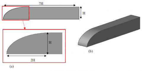
In the present article, a simplified model of high-speed train is used. Since practical and real high-speed trains have complicated geometries, they are not used for aerodynamic analysis. Instead, the simplified high-speed train can be used in both numerical and experimental research.
The train model that was used in the present paper is a simplified one which applied in previous research by Sakuma et al. [27], Ishak et al. [28] and Hemida et al. [29]. Figure 2 indicates that the geometry of the simplified high-speed train. The geometric specifications of the train are also as Figure 2.
Figure 2. Side view (a), and isometric view (b) of the simplified high-speed train
3.2 Domain description
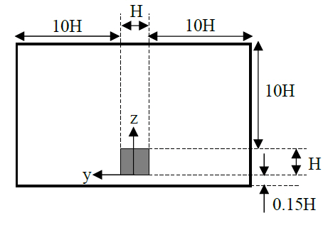
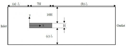
As Figures 3, 4 and 5, the side, front and top views of the high-speed train and the exact location of the high-speed train in the computational domain are shown, respectively [27-29].
Figure 3. Side view of the high-speed train and the exact location of the high-speed train in the computational domain
Figure 4. Front view of the high-speed train and the exact location of the high-speed train in the computational domain
Figure 5. Top view of the high-speed train and the exact location of the high-speed train in the computational domain
3.3 Mesh description
The cells in the numerical simulation are generated via a structured non-uniform Cartesian mesh by blockMesh, that is a basic meshing tool in the OpenFOAM. Further mesh refinement is applied close to the train body and its around areas using the mesh generation utility of the SnappyHexMesh tool, which is also supplied with the OpenFOAM. Due to evaluate the results and the effects of the vortex structure close to the train body and increase the accuracy of numerical simulation, the two different types of computational grids are designed: a grid with large nodes and the other with small nodes. The type of the grid around the train and especially close to the surface is hexahedral and due to reduced computational volume of the CPU, the grid in the farther area of the train is designed as tetrahedral. The different grid resolutions are selected according to grid refinement ratio, r. According to [24], it is favorable that the grid refinement ratio to be greater than 1.3. In this model, r=1.4 is selected (Eq. (4)). The grid refinement ratio is estimated according to average grid size (have) as shown in Eqns. 5 and 6. More details of them can be seen in Table 1. The grid refinement ratio, r and is calculated as follows:
$r=\frac{h_{\text {ave }} \text { (large grid) }}{h_{\text {ave }}(\text { small grid) }}$ (4)
$2 D$ Computation $-h_{\text {ave }}=\left[\frac{1}{N} \sum_{i=1}^{N}\left(\Delta A_{i}\right)\right]^{\frac{1}{2}}$ (5)
$3 D$ Computation $-h_{\text {ave }}=\left[\frac{1}{N} \sum_{i=1}^{N}\left(\Delta V_{i}\right)\right]^{\frac{1}{3}}$ (6)
where, $\Delta V_{i}$ and $\Delta A_{i}$ are the volume and the area of the ith cell, respectively and N is the total number of cells used for the computations. Also, to reduce the computational volume, wall functions are used in cells close to the surface. Moreover, the $y^{+}$ range is between 80 and 90 for these cases. Also, the mesh details around the train and the two refinement boxes close the train is shown in Figure 6. Finally, Figure 7 illustrates the residual error for different parameters of the paper. According to this figure, all values and parameters used in the numerical calculation are converged.
Figure 6. Mesh details around the train and the two refinement boxes close the train
Figure 7. Residual error for different parameters
Table 1. Details of the grid resolutions
|
Case |
Large Grid |
Small Grid |
|
Total no. of cells |
780,505 |
3,456,788 |
|
Cell size, ℎave |
0.1361 |
0.07886 |
|
Averaged y+ |
98.4 |
83.7 |
|
Refinement ratio, r |
1.4 |
1.4 |
3.4 Boundary conditions (B.C.)
The specified boundary conditions for the case are shown in Table 2:
Table 2. Specified boundary conditions for this case
|
B.C. |
Description |
|
Inlet |
Uniform velocity in the x-direction (U∞) |
|
Outlet |
Homogenous Neumann (grad. P = 0) |
|
Side & Top |
Patch type with a freestream value |
|
Ground |
wall boundary condition (no-slip) |
|
Train |
wall boundary condition (no-slip) |
Also, the air flow specifications are listed in Table 3.
Table 3. Air flow specifications
|
Parameter |
Value |
|
Reynolds number (Re) |
2.6 × 10⁶ |
|
Free stream velocity (U∞) |
70 m/s |
|
kinematic viscosity (ν) |
1.5 × 10⁻⁵ m2/s |
|
H |
0.56 m |
3.5 Solution methodology and governing equations
To solve this problem, an incompressible, three-dimensional and turbulent air flow around the train is considered. In the following, combining Reynolds-Averaged Navier-Stokes (RANS) with the $k-\omega$ SST turbulence methods, the problem of the air flow around the train is solved. The RANS method, is a time-average one of description of air flow. In the RANS method, regular quantities are replaced with oscillating and average ones. The OpenFOAM CFD software package is applied to solve the governing equations.
Based on the solution approach, the continuity and Navier-Stokes equations are as follows:
$\frac{\partial u_{i}}{\partial x_{j}}=0$ (7)
$\rho \frac{\partial u_{i}}{\partial x_{j}}+\rho U_{j} \frac{\partial u_{i}}{\partial x_{j}}=-\frac{\partial p_{i}}{\partial x_{j}}+\frac{\partial}{\partial x_{j}}\left[\mu\left(\frac{\partial u_{j}}{\partial x_{j}}+\frac{\partial u_{i}}{\partial x_{j}}\right)\right]$ (8)
where, i, j = 1, 2, 3 are related to the x–, y– and z–directions in a Cartesian coordinate system, respectively. The velocity and pressure components, $u_{i}$ and $p_{i}$ are nonlinear. The instability of the flow parameters (i.e., pressure and velocity) are disintegrated into mean value and fluctuations as follows:
$u_{i}=U_{i}+u_{i}^{\prime}$ (9)
$p_{i}=P_{i}+p_{i}^{\prime}$ (10)
where, $U_{i}$ and $P_{i}$ are the time-averaged values, while $u_{i}^{\prime}$ and $p_{i}^{\prime}$ are the fluctuation terms of them, respectively. Substituting the Reynolds disintegrated velocities and pressures into the Navier-Stokes and Continuity equations yields the Reynolds Averaged Navier-Stokes equation of motions as illustrated below:
$\frac{\partial U_{i}}{\partial x_{j}}=0$ (11)
$\frac{\partial U_{i}}{\partial t}+U_{j} \frac{\partial U_{i}}{\partial x_{j}}=-\frac{1}{\rho} \frac{\partial P_{i}}{\partial x_{i}}+\frac{\partial}{\partial x_{j}}\left(\mu \frac{\partial U_{i}}{\partial x_{j}}-\rho \overline{u_{l}^{\prime} u_{j}^{\prime}}\right)$ (12)
Based on the Boussinesq, the tensor of the Reynolds-stress could be joint to the mean rate of deformation. The turbulent concept model which applied is as follow:
$-\rho \overline{u_{l}^{\prime} u_{j}^{\prime}}=\mu_{t}\left(\frac{\partial U_{i}}{\partial x_{j}}+\frac{\partial U_{j}}{\partial x_{i}}-\frac{2}{3} \frac{\partial U_{k}}{\partial x_{k}} \delta_{i j}\right)-\frac{2}{3} \rho k \delta_{i j}$ (13)
Also, the specific dissipation rate (ω) as follow:
$\begin{aligned} \frac{\partial \omega}{\partial t}+U_{j} \frac{\partial \omega}{\partial x_{j}}=\alpha S^{2}-& \beta \omega^{2}+\frac{\partial}{\partial x_{j}}\left[\left(v+\sigma_{\omega} v_{T}\right) \frac{\partial \omega}{\partial x_{j}}\right] \\+2\left(1-F_{1}\right) \sigma_{\omega 2} \frac{1}{\omega} \frac{\partial k}{\partial x_{i}} \frac{\partial \omega}{\partial x_{i}} \end{aligned}$ (14)
where, vT is the kinematic eddy viscosity and can be described as follows:
$v_{T}=\frac{\alpha_{1} k}{\max \left(\alpha_{1} \omega, S F_{2}\right)}$ (15)
The following closure coefficient is applied in the research:
$F_{2}=\tanh \left[\left[\max \left(\frac{2 \sqrt{k}}{\beta^{*} \omega y}, \frac{500 v}{y^{2} \omega}\right)\right]^{2}\right]$ (16)
where, y is the space to the next surface,
$P_{k}=\min \left(\tau_{i j} \frac{\partial U_{i}}{\partial x_{j}}, 10 \beta^{*} k \omega\right)$ (17)
$F_{1}=\tanh \left\{\left\{\min \left[\max \left(\frac{\sqrt{k}}{\beta^{*} \omega y}, \frac{500 v}{y^{2} \omega}\right), \frac{4 \sigma_{\omega 2} k}{C D_{k \omega} y^{2}}\right]\right\}^{4}\right\}$ (18)
$C D_{k \omega}=\max \left(2 \rho \sigma_{\omega 2} \frac{1}{\omega} \frac{\partial k}{\partial x_{i}} \frac{\partial \omega}{\partial x_{i}}, 10^{-10}\right)$ (19)
$\phi=\phi_{1} F_{1}+\phi_{2}\left(1-F_{1}\right)$ (20)
$\alpha_{1}=\frac{5}{9}, \quad \alpha_{2}=0.44$ (21)
$\beta_{1}=\frac{3}{40}, \quad \beta_{2}=0.0828, \quad \beta^{*}=\frac{9}{100}$ (22)
$\sigma_{k 1}=0.85, \sigma_{k 2}=1, \sigma_{\omega 1}=0.5, \sigma_{\omega 1}=0.856$, (23)
The most important and most useful aerodynamic components and parameters for simulation of bluff bodies, especially high-speed trains are drag, lift and side forces. To achieve this, the aerodynamic forces for the train for various wind directions are calculated, clearly. The lift, drag and side coefficients are defined as follows:
3.6 Aerodynamic forces
$C_{L}=\frac{F_{L}}{\frac{1}{2} \rho U_{\infty}^{2} A_{L}}$ (24)
$C_{D}=\frac{F_{D}}{\frac{1}{2} \rho U_{\infty}^{2} A_{D}}$ (25)
$C_{S}=\frac{F_{S}}{\frac{1}{2} \rho U_{\infty}^{2} A_{S}}$ (26)
where, $F_{L}, F_{D}$ and $F_{S}$ are the lift, drag and side forces, $A_{L}, A_{D}$ and $A_{S}$ are the surface of the train in z-, x- and y-directions, respectively. Moreover, the coefficient of pressure is as follow:
$C_{P}=\frac{P-P_{\infty}}{\frac{1}{2} \rho U_{\infty}^{2}}$ (27)
where, $P_{\infty}, U_{\infty}$ and $\rho$ are the free stream pressure and velocity and density, respectively.
In this section, the first, effects of yaw angles change on the aerodynamic coefficients of air flow around the high-speed train are performed. Then, the effects of wall functions changes on aerodynamic behavior of air turbulent flow around the high-speed train are provided.
For different yaw angles of this research, i.e., 0˚, 30˚, 45˚ and 60˚ and for 70 m/s free stream velocity, the lift, drag and side aerodynamic coefficients are compared which are illustrated in Table 4. As can be seen from Table 4, when the yaw angle increase, the lift, drag and side aerodynamic coefficients increase. Then, the friction and resistance against train movement increase too. Moreover, in Table 5, the minimum, maximum and average values of the pressure coefficients for mentioned different yaw angles are listed and compared. As the same way, with increasing the yaw angle of the free stream, the numerical values of the minimum, maximum and the average values of the pressure coefficients increase too. Also, the maximum value of pressure coefficient at 60˚ yaw angle has the highest value.
Table 4. Aerodynamic force coefficients for yaw angles
|
Aerodynamic Coeffs. (U∞ = 70 m/s) |
CL |
CD |
CS |
|
0° |
0.34 |
0.48 |
0.01 |
|
30° |
0.90 |
0.71 |
2.15 |
|
45° |
1.06 |
0.93 |
2.61 |
|
60° |
1.63 |
1.42 |
3.02 |
Table 5. Minimum, maximum and average pressure coefficients for different yaw angles
|
Pressure Coeffs. (U∞ = 70 m/s) |
CP,min |
CP,max |
CP,ave |
|
0° |
-1.91 |
0.98 |
-0.10 |
|
30° |
-4.10 |
2.88 |
-0.03 |
|
45° |
-6.72 |
4.56 |
-0.40 |
|
60° |
-8.70 |
4.66 |
-0.33 |
a) Wall functions used for turbulent kinetic energy, k:
kqRWallFunction: This wall function provides Neumann boundary condition.
v2WallFunction: This wall function provides the stress normal to streamlines boundary condition. v2 is calculated in the non-dimensional form.
kLowReWallFunction: This wall function establishes a boundary condition of turbulence kinetic energy for high- and low- Reynolds number turbulent flows. Also, it can provide boundary condition if the first cell center is placed in buffer layer.
omegaWallFunction: According to the mentioned theory mentioned, this wall function presents the composition of log equation and viscous. In the OpenFOAM, this wall function is a specific wall function that can exchange between logarithmic and viscous regions based on the position of y+. In the junction of the log-law region and viscous sublayer values is estimated via blending the viscous and log-law sublayer value.
In the following, first, the velocity and the pressure contours of air flow around the high-speed train for some wall functions (the wall functions are used for the kinetic energy) are displayed and compared. Then comparisons between wall functions (the wall functions are used for turbulence viscosity) and for Enhanced Wall Functions on aerodynamic key parameters as drag, lift and side forces and pressure coefficients are performed and Also, the CPU times of each cases are listed and compared.
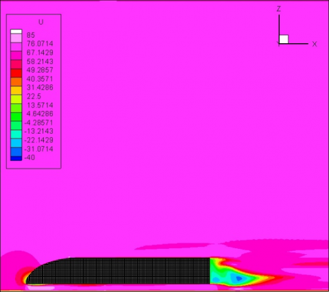
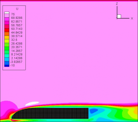
Figures 8-11 represents the 2D velocity contour (x-direction velocity: U) around the high-speed train for four mentioned used wall functions which applied for turbulent kinetic energy. Figures 8, 9, 10 and 11 show the velocity contour around the train using kqRWallFunction, v2WallFunction, kLowReWallFunction and omegaWallFunction, respectively. As can be seen, the 2D velocity contour around the train for mentioned four cases are not the same and minor different are observed. According to the previous finding and principal data, omegaWallFunction case has most deviation compared with the expected results. However, the results of the three other cases (kqRWallFunction, v2WallFunction and kLowReWallFunction) are almost identical and are suitable for describing the velocity contour.
Figure 8. Velocity profile of the train gained from kqRWallFunction
Figure 9. Velocity profile of the train gained from v2WallFunction
Figure 10. Velocity profile of the train gained from kLowReWallFunction
Figure 11. Velocity profile of the train gained from omegaWallFunction
Figure 12. Pressure profile of the train gained from kqRWallFunction
Figure 13. Pressure profile of the train gained from v2WallFunction
In the following, the 2D pressure contour around the train for the mentioned wall function cases of turbulent kinetic energy is illustrated in Figures 12-15. As expected, the maximum value of the pressure occurs at the nose of the train and the minimum value of it is located at the back of the train. kqRWallFunction, v2WallFunction, kLowReWallFunction and omegaWallFunction are used for describing pressure contour around the train in Figures 12, 13, 14 and 15, respectively. Similarly, the first three cases are more suitable than the last wall function case. Based on the two series of results (velocity and pressure contours), kqRWallFunction, v2WallFunction and kLowReWallFunction cases of wall functions are more accurate than omegaWallFunction case of wall function for flow analysis around the train.
Then, the exact pressure coefficient for wall functions changes for different regions on the train surface as Figure 16 is shown in Figure 17. As shown in Figure 17, the pressure coefficients of the train surface for four kinds of wall functions related to the turbulent kinetic energy were illustrated, separately. The desired values are listed in Figure 16 based on the marked points.
The pressure coefficient at the beginning and the end of the train are higher than the other regions of the train body. The maximum value of pressure coefficient occurs at the beginning of the train and the minimum one occurs at the middle of the train surface.
Figure 14. Pressure profile of the train gained from kLowReWallFunction
Figure 15. Pressure profile of the train gained from omegaWallFunction
Figure 16. The nodes of train surface for pressure coefficient in Figure 14
Figure 17. Pressure coefficients for different regions on the train surface
b) Wall functions used for turbulence viscosity, νt:
nutkWallFunction: This wall function presents a turbulence viscosity condition according to the turbulence kinetic energy.
nutUWallFunction: The structure of this class is almost similar to last wall function.
nutLowReWallFunction: This wall function sets the turbulence viscosity into zero.
nutUSpaldingWallFunction: This wall function is based on the special relationship between y+ and u+. Also, the curve can fit on u+ = y+ curve in the viscous layer.
EnhancedWallFunction:
ANSYS FLUENT company in order to create a wall function is corrected in all areas along the wall (i.e., viscous sublayer region, buffer and fully-turbulent outer regions) was provided Enhanced Wall Function. This wall function merges the relationships between the laminar and logarithmic regions (turbulent) with a blending function and therefore is correct in all areas along the wall. In many turbulence cases, the y+ is not the first uniform cell, therefore the selection of the appropriate wall function is difficult. The superiority of this wall function is that it supports all the values of y+ and can be used in surfaces with heterogeneous distribution of y+. OpenFOAM software, due to its object-oriented nature, is a suitable tool for code development and comparison of various numerical methods. For this reason, after developing the code for the Enhanced Wall Functions in this software, it is compared with the default open-source functions.
To verify the results of the article, an approximate comparison has been made between the results of this article and the Ref. [19]. The used geometries and the computational domains in the simulation are almost identical in the two articles. The comparison results are shown in Table 6. Also, the comparison results for 20 m/s are shown in Table 6. Also, the minimum and maximum differences between these results are about 0 to 16 percent, respectively.
Table 6. Comparison of time-averaged values between the paper and the Ref. [19]
|
Cases 20 m/s |
This paper |
Ref. 19 |
||
|
CL |
CS |
CL |
CS |
|
|
θ = 30° |
0.113 |
0.407 |
0.136 |
0.424 |
|
θ = 60° |
0.170 |
1.042 |
0.161 |
1.029 |
In the Following, for 70 m/s velocity, three categories of comparison are done:
A comparison on aerodynamic forces (drag, lift and side) for different wall functions used in turbulent viscosity which is shown in Table 7. In this table, drag, lift and side aerodynamic coefficients for four used wall functions of turbulent viscosity as nutkWallFunction, nutUWallFunction, nutLowReWallFunction, nutUSpaldingWallFunction and EnhancedWallFunction are compared and a comparison with a similar numerical research (Ref. [19]) is verified. Based on Table 7, all used wall functions have fairly accurate results and EnhancedWallFunction has closest results to Ref. [19]. The aerodynamic coefficients (drag, lift and side) by EnhancedWallFunction which implemented from ANSYS FLUENT into OpenFOAM obtained good and relatively accurate results.
Table 8 is similar to Table 7 with this difference that instead of aerodynamic coefficients, the pressure coefficients as pressure coefficient at maximum, minimum and average values are compared for the mentioned wall functions used for turbulent viscosity. As specified in the table, EnhancedWallFunction and nutkWallFunction have closest results to Ref. [19] again although the other wall functions have relatively acceptable results.
Table 7. Comparison of aerodynamic forces for different wall functions of turbulent kinetic energy
|
Wall Functions |
CD |
CL |
CS |
|
nutkWallFunction |
0.776 |
-0.339 |
0.00395 |
|
nutUWallFunction |
0.728 |
-0.342 |
0.00356 |
|
nutLowReWallFunction |
0.676 |
-0.337 |
0.00405 |
|
nutUSpaldingWallFunction |
0.724 |
-0.343 |
0.00377 |
|
EnhancedWallFunction |
0.778 |
-0.339 |
0.00393 |
|
Ref. [19] |
0.780 |
-- |
-- |
Table 8. Comparison of pressure coefficients for different wall functions of turbulence viscosity
|
Wall Functions |
CP,min |
CP,max |
CP,ave |
|
nutkWallFunction |
-1.614 |
0.995 |
-0.095 |
|
nutUWallFunction |
-1.890 |
0.993 |
-0.098 |
|
nutLowReWallFunction |
-1.914 |
0.983 |
-0.104 |
|
nutUSpaldingWallFunction |
-1.892 |
0.992 |
-0.097 |
|
EnhancedWallFunction |
-1.402 |
1.003 |
-0.097 |
|
Ref. [19] |
-1.301 |
1.010 |
-0.093 |
In Tables 9 and 10, the computational times of CPU for two series of wall functions (used for turbulent kinetic energy and turbulence viscosity) are shown. Based on the tables, kqRWallFunction and EnhancedWallFunction for turbulent kinetic energy and EnhancedWallFunction for turbulence viscosity have minimum CPU times.
Table 9. Comparison of CPU time for different wall functions of turbulent kinetic energy
|
Wall Functions |
CPU Time (sec) |
|
kqRWallFunction |
10,742 |
|
V2WallFunction |
10,779 |
|
kLowReWallFunction |
10,813 |
|
omegaWallFunction |
10,776 |
|
EnhancedWallFunction |
10,569 |
Table 10. Comparison of CPU time for different wall functions of turbulence viscosity
|
Wall Functions |
CPU Time (sec) |
|
nutkWallFunction |
10,691 |
|
nutUWallFunction |
10,746 |
|
nutLowReWallFunction |
10,812 |
|
nutUSpaldingWallFunction |
10,799 |
|
EnhancedWallFunction |
10,691 |
In the present research, the effects of some practical wall functions on the description of air flow and aerodynamic parameters for a simplified high-speed train are investigated. To achieve this, combining Reynolds-Averaged Navier-Stokes equation with the k-ω SST turbulence approach are used to solve the governing equations of the problem. Also, the OpenFOAM software is applied to more accurate simulation of turbulent air flow around the mentioned high-speed train. In addition, the pressure and velocity contours around the train for four common wall functions of turbulent kinetic energy are analyzed. In the following, the aerodynamic drag, lift and side coefficients and pressure for four common wall functions and for a new improvement wall function called Enhanced Wall Functions used for turbulence viscosity are compared and investigated. Finally, the CPU times for the mentioned wall functions are listed. In these comparisons, the most appropriate wall function in terms of accuracy is suggested and selected.
Based on the simulation findings, in turbulent kinetic energy comparison, the implemented wall function (EnhancedWallFunction) has the closest result with the validation article and the most accurate one. In the turbulent viscosity comparison, EnhancedWallFunction and nutkWallFunction showed the best results. Moreover, in terms of computational time, kqRWallFunction and EnhancedWallFunction for turbulent kinetic energy and EnhancedWallFunction for turbulence viscosity have minimum CPU times.
Generally, the implemented wall function (EnhancedWallFunction) makes more accurate results and is valid in all areas along the wall. The findings depicted the capability of the proposed approach for the numerical analysis of turbulent air flow around the simplified high-speed train. The successful implementation of the approach indicates its efficiency, generality and flexibility. The CFD OpenFOAM toolbox demonstrated to be a very useful tool for turbulent flows.
|
AD |
surface of the train in y-direction |
|
AL |
surface of the train in z-direction |
|
AS |
surface of the train in x-direction |
|
CD |
aerodynamic drag coefficient |
|
CL |
aerodynamic lift coefficient |
|
CP |
aerodynamic pressure coefficient |
|
CS |
aerodynamic side coefficient |
|
FD |
aerodynamic drag force |
|
FL |
aerodynamic lift force |
|
FS |
aerodynamic side force |
|
have |
average grid size |
|
k |
turbulent kinetic energy |
|
P |
time-averaged pressure |
|
p |
pressure |
|
p' |
fluctuation terms of pressure |
|
P∞ |
free stream pressure |
|
r |
grid refinement ratio |
|
Re |
Reynolds number |
|
U |
time-averaged velocity |
|
u |
velocity |
|
u’ |
fluctuation terms of velocity |
|
U∞ |
free stream velocity |
|
u* |
velocity of flow near wall region |
|
u+ |
non-dimensional velocity |
|
y |
distance to wall |
|
y+ |
non-dimensional length |
|
Greek symbols |
|
|
θ |
yaw angle of air flow |
|
ρw |
density of wall |
|
υ |
kinematic viscosity |
|
νt |
turbulence viscosity |
|
τw |
shear stress of wall |
[1] Patankar, S.V., Spalding, D.B. (1970). Heat and Mass Transfer in Boundary Layers. 2nd ed. London: Intertext Books. https://doi.org/10.1017/S0022112071212532
[2] Rashidi, M.M., Hajipour, A., Li, T., Yang, Z., Li, Q. (2019). A Review of recent studies on simulations for flow around high-speed trains. Journal of Applied and Computational Mechanics, 5(2): 311-333. https://doi.org/10.22055/JACM.2018.25495.1272
[3] Paradot, N., Talotte, C., Garem, H., Delville, J., Bonnet, J.P. (2002). A comparison of the numerical simulation and experimental investigation of the flow around a high speed train. ASME 2002 Fluids Engineering Division Summer Meeting Montreal, Quebec, Canada, pp. 1055-1060. http://dx.doi.org/10.1115/FEDSM2002-31430
[4] Khier, W., Breuer M., Durst, F. (2002). Numerical computation of 3-D turbulent flow around high-speed trains under side wind conditions. TRANSAERO - A European Initiative on Transient Aerodynamics for Railway System Optimisation, 79: 75-86. http://dx.doi.org/10.1007/978-3-540-45854-8_7
[5] Fauchier, C., Le Devehat, E., Gregoire, R. (2002). Numerical study of the turbulent flow around the reduced-scale model of an Inter-Regio. TRANSAERO - A European Initiative on Transient Aerodynamics for Railway System Optimisation, 79: 61-74. http://dx.doi.org/10.1007/978-3-540-45854-8_6
[6] Shin, C.H., Park, W.G. (2003). Numerical study of flow characteristics of the high speed train entering into a tunnel. Mechanics Research Communications, 30(4): 287-296. http://dx.doi.org/10.1016/S0093-6413(03)00025-9
[7] Tian, H. (2009). Formation mechanism of aerodynamic drag of high-speed train and some reduction measures. Journal of Central South University of Technology, 16: 166-171. http://dx.doi.org/10.1007/s11771-009-0028-0
[8] Zhao, J., Li, R. (2009). Numerical analysis for aerodynamics of high- speed trains passing tunnels. The Aerodynamics of Heavy Vehicles II: Trucks, Buses, and Trains, 41: 239-239. http://dx.doi.org/10.1007/978-3-540-85070-0_23
[9] Krajnović, S. (2009). Optimization of aerodynamic properties of high-speed trains with CFD and response surface models. The Aerodynamics of Heavy Vehicles II: Trucks, Buses, and Trains, 41: 197-211. http://dx.doi.org/10.1007/978-3-540-85070-0_16
[10] Li, X., Deng, J., Chen, D., Xie, F., Zheng, Y. (2011). Unsteady simulation for a high-speed train entering a tunnel. Journal of Zhejiang University-SCIENCE A, 12: 957-963. http://dx.doi.org/10.1631/jzus.A11GT008
[11] Wang, D., Li, W., Zhao, W., Han, H. (2012). Aerodynamic numerical simulation for EMU passing each other in tunnel. Proceedings of the 1st International Workshop on High-Speed and Intercity Railways, 2: 143-153. http://dx.doi.org/10.1007/978-3-642-27963-8_15
[12] Östh, J., Krajnović, S. (2012). Simulations of flow around a simplified train model with a drag reducing device. The 15th International Conference on Fluid Flow Technologies Budapest, Hungary. http://publications.lib.chalmers.se/publication/163187
[13] Asress, M.B., Svorcan, J. (2014). Numerical investigation on the aerodynamic characteristics of high-speed train under turbulent crosswind. Journal of Modern Transportation, 22(4): 225-234. http://dx.doi.org/10.1007/s40534-014-0058-7
[14] Peng, L., Fei, R., Shi, C., Yang, W., Liu, Y. (2014). Numerical simulation about train wind influence on personnel safety in high-speed railway double-line tunnel. Parallel Computational Fluid Dynamics, 405: 553-564. http://dx.doi.org/10.1007/978-3-642-53962-6_50
[15] Shuanbao, Y., Dilong, G., Zhenxu, S., Guowei, Y., Dawei, C. (2014). Optimization design for aerodynamic elements of high speed trains. Computers & Fluids, 95(22): 56-73. http://dx.doi.org/10.1016/j.compfluid.2014.02.018
[16] Chu, C.R., Chien, S.Y., Wang, C.Y., Wu, T.R. (2014). Numerical simulation of two trains intersecting in a tunnel. Tunnelling and Underground Space Technology, 42: 161-174. http://dx.doi.org/10.1016/j.tust.2014.02.013
[17] Zhang, J., Gao, G., Liu, T., Li, Z. (2015). Crosswind stability of high-speed trains in special cuts. Journal of Central South University, 22: 2849-2856. http://dx.doi.org/10.1007/s11771-015-2817-y
[18] Morden, J.A., Hemida H., Baker, C.J. (2015). Comparison of RANS and detached eddy simulation results to wind-tunnel data for the surface pressures upon a class 43 high-speed train. Journal of Fluids Engineering, 137(4). http://dx.doi.org/10.1115/1.4029261
[19] Zhuang, Y., Lu, X. (2015). Numerical investigation on the aerodynamics of a simplified high-speed train under crosswinds. Theoretical and Applied Mechanics Letters, 5(5): 181-186. http://dx.doi.org/10.1016/j.taml.2015.06.001
[20] Catanzaro, C., Cheli, F., Rocchi, D., Schito, P., Tomasini, G. (2016). High-speed train crosswind analysis: CFD study and validation withwind-tunnel tests. The Aerodynamics of Heavy Vehicles III, 79: 99-112. http://dx.doi.org/10.1007/978-3-319-20122-1_6
[21] Ding, S., Li, Q., Tian, A., Du, J., Liu, J. (2016). Aerodynamic design on high-speed trains. Acta Mechanica Sinica, 32(2): 215-232. http://dx.doi.org/10.1007/s10409-015-0546-y
[22] Liu, T.H., Su, X.C., Zhang, J. (2016). Aerodynamic performance analysis of trains on slope topography under crosswinds. Journal of Central South University, 23: 2419-2428. http://dx.doi.org/10.1007/s11771-016-3301-z
[23] Premoli, A., Rocchi, D., Schito, P., Tomasini, G. (2016). Comparison between steady and moving railway vehicles subjected to crosswind by CFD analysis. Journal of Wind Engineering and Industrial Aerodynamics, 156: 29-40. http://dx.doi.org/10.1016/j.jweia.2016.07.006
[24] Jia, Y., Mei, Y. (2018). Numerical simulation of pressure waves induced by high-speed maglev trains passing through tunnels. International Journal of Heat and Technology, 36(2): 687-696. http://dx.doi.org/10.18280/ijht.360234
[25] Li, T., Zhang, J., Rashidi, M., Yu, M. (2019). On the reynolds-average navier-stokes modelling of the flow around a simplified train in crosswinds. Journal of Applied Fluid Mechanics, 12(2): 551-563. http://doi.org/10.29252/jafm.12.02.28958
[26] Li, T., Hemida, H., Rashidi, M.M., Zhang, W. (2020). The effect of numerical divergence schemes on the flow around trains. Fluid Dynamics Research, 52(2). http://dx.doi.org/10.1088/1873-7005/ab8314
[27] Sakuma, Y., Ido, A. (2009). Wind tunnel experiments on reducing separated flow region around front ends of vehicles on meter-gauge railway lines. Quarterly Report of RTRI, 50(1): 20-25. http://dx.doi.org/10.2219/rtriqr.50.20
[28] Ishak, I.A., Ali, M.S.M., Yakub M.F.M., Salim, S.A.Z.S. (2019). Effect of crosswinds on aerodynamic characteristics around a generic train model. International Journal of Rail Transportation, 7(1): 23-54. http://dx.doi.org/10.1080/23248378.2018.1424573
[29] Hemida, H., Krajnović, S. (2010). LES study of the influence of the nose shape and yaw angles on flow structures around trains. Journal of Wind Engineering and Industrial Aerodynamics, 98: 34-46. http://dx.doi.org/10.1016/j.jweia.2009.08.012