Khelifa Hami
© 2021 IIETA. This article is published by IIETA and is licensed under the CC BY 4.0 license (http://creativecommons.org/licenses/by/4.0/).
OPEN ACCESS
This contribution represents a critical view of the advantages and limits of the set of mathematical models of the physical phenomena of turbulence. Turbulence models can be grouped into two categories, depending on how turbulent quantities are calculated: direct numerical simulations (DNS) and RANS (Reynolds Averaged Navier-Stokes Equations) models. The disadvantage of these models is that they require enormous computing power, inaccessible, especially for large and complicated geometries. For this reason, hybrid models (combinations between DNS and RANS methods) have been developed, for example, the LES (“Large Eddy Simulation”) or DES (“Detached Eddy Simulation”) models. They represent a compromise - are less precise than DNS, but more precise than RANS models. The results presented in this contribution will allow and facilitate future research in the field the choice of the model approach necessary for the case studies whatever their difficulty factor.
turbulence models, RANS, LES, DNS, CFD applications
Numerical simulation can be of great help for research, since analytical computation remains very ineffective here. However, it would be imprudent to consider this approach as the only route to take; indeed, the modeling of flows rather complements tests on site or on a model.
During a study, the CFD often intervenes upstream during the design and then avoids the manufacturers to manufacture many and above all expensive prototypes. It can then be characterized as “virtual prototyping”. In fact, one of the main advantages of numerical computation is the possibility of varying the geometric, dynamic or thermo-physical parameters of the problem being treated by avoiding the repetition of long and cumbersome experiments to manage. Then, further downstream of the study, it can be useful for analyzing damage detected on equipment or for improving its performance.
CFD ("Computational Fluid Dynamics") is a branch of fluid mechanics that uses numerical methods and algorithms to analyze and solve problems that involve moving fluids. In short, the differential equations that govern the transport of mass, momentum, turbulent variables and energy are solved numerically.
Nowadays, a CFD is a very powerful tool, often used in several industrial and research fields. Under certain conditions, it can supplement and even replace experimental investigations.
In the case of problems whose mathematical model is not yet sufficiently developed, (it contains approximations, uncertainties - for example the RANS models of turbulence); the CFD can be used only after an experimental validation. This comparison is necessary to establish the degree of agreement between the numerical results and reality.
Comparison with experimental investigations, the CFD offers a series of advantages:
Reduced cost, especially when the digital model replaces a large or very complicated physical model.
Velocity: numerical simulation can be very fast. Several configurations of a model can be studied, and compared in a single day. An experimental investigation would take much longer.
Complete information: all the variables of a problem (velocity, temperature, pressure, etc.) are available everywhere in the calculation domain, whereas, in the case of an experiment, there are several inaccessible places for measuring instruments. The ability to simulate conditions difficult to reach by experiments: very small or very large models, very high or very low temperatures, very slow or very fast processes.
Possibility of idealizing: in some simulations, we want to focus on a few essential parameters and eliminate others that are not relevant.
In this work, we review some themes that have captured the attention of the international scientific community for more than three decades. Generally speaking, the coupling of the differential equations "momentum, energy equation, etc." makes the study problems very delicate.
In this part, we will present some results for geometries commonly encountered in housing: case of the flat plate and "rectangular" cavities, 2D, and 3D. Of all the problems, it is that of convection along a flat plate subjected either to a constant flux density or to a constant temperature, which has been the object of the most important works, both theoretical and experimental.
This classification delimits three flow zones as a function of Re. In addition, it can be noted that if the limit between laminar and transient regime is fairly well defined, that between the transient and the turbulent is still poorly understood [1].
In the laminar regime, the fluid threads remain parallel to each other and the flow is characterized by its great stability. In this simple case, the transfer, theoretically evaluated by numerical or analytical methods, then verified experimentally [2].
The transition from laminar to turbulent Figure 1. It is characterized by the appearance of slight deformations of the fluid threads, witnesses of thermal fluctuations of large amplitude. Attempts, very numerous, to study the characterization of this area; still pose great difficulties because the experimental approach is very delicate.
Figure 1. The uniform velocity profile for the transition between the laminar and turbulent regions
The development of numerical analysis techniques makes it possible to better model the phenomena of natural convection from basic equations, for simple boundary conditions such as the isothermal flat plate immersed in a fluid medium. Numerical diagrams exist and allow the simulation of the Navier-Stocks equations. However, the latter can no longer be used once the flows become turbulent.
In the case of cavities, additional hypotheses and therefore additional equations are to be taken into account in the resolutions, and the problems quickly become very complicated. This is certainly one of the reasons why the results of flat plates have long served as a comparison element for natural convection flows in confined spaces (cavities).
Xin and Le Quéré [1] designate the differentially heated cavity as being a closed rectangular enclosure of which two opposite vertical walls are subjected to a constant temperature difference, the other adiabatic walls, and the vertical aspect ratio is between 0.5 and 10.
The visualizations carried out by the authors reveal the stable nature of the laminar boundary layer flow near the vertical wall, even for the Grashof amount of the order of 1011. However, this stable flow remains very fragile; indeed, a minimal modification of the boundary conditions leads to a strong destabilization of the flows near the walls, leading to a significant increase in local flow densities.
From the point of view of numerical simulation, we are witnessing today the emergence of several calculation methods to characterize the turbulent flows, Tian and Karayiannis [2] for DNS. Peng and Davidson [3], Sergentet et al. [4], Ezzouhri et al. [5] for LES, Hami et al. [6, 7]and others by RANS ("Reynolds Averaged Navier-Stokes Equations").
Recent work has been published on the application of these methods:
A realizable k–ε turbulence model of an incompressible fluid is extended for the stable atmosphere after taking account of the buoyancy damping of gravity waves [8]. The new model is consistent with the Monin–Obukhov similarity theory on the stable atmospheric boundary layer (ABL) over a horizontally uniform surface. The model is incorporated into an ABL model to simulate mean flow against observations. Its ABL-model output is compared with the Leipzig dataset, showing the turbulence model works well for a stable ABL. Specifically, the ABL model properly replicates 1) the mixing length, turbulent viscosity, and mean wind; 2) a significant decrease of the mixing length with height in the upper ABL and thus a reasonable altitude of the ABL top; and 3) a sensitivity of the mixing length and turbulent viscosity to atmospheric stability.
The paper [9] reviews in condensed form and from a historical perspective the various methods for treating and simulating turbulence and its effects in hydraulic flows. After highlighting the main characteristic features of turbulence and the role it plays in hydraulics, a necessarily brief overview is given of the main methods used in hydraulic flow calculations for dealing with turbulence and its effects. These are (1) empirical relations, (2) methods solving the Reynolds-averaged Navier-Stokes (RANS) equations with the aid of statistical turbulence models, (3) direct numerical simulations (DNS), and (4) large-eddy simulations (LES). Brief comments are made on the historical development of the different methods, and for RANS, DNS, and LES methods some application examples are presented. For details on the individual methods and further application examples, the reader is directed to the very extensive literature.
Turbulent flow in Z-shape duct configuration is investigated using Reynolds stress model (RSM) and ζ-f model and compared to experimental results [10]. Both RSM and ζ-f models are based on steady-state RANS solutions. The focus was on regions where the RSM has over- or underpredicted the flow when compared to the experimental results and on regions where there are flow separations and high turbulence. The performance of predicting the flow reattachment length in each model is studied as well. RSM has shown the mean flow velocity profile results match reasonably well with the experiment. Advanced ζ-f turbulence model is introduced as user-defined function (UDF) code and applied to the Z-shape duct. It is found that the turbulent kinetic energy production in ζ equation is much easier to reproduce accurately. Both mean velocity gradient and local turbulent stress terms are also much easier to be resolved properly.
To define the state of a moving fluid, for unknown functions must be determined: the three components of the velocity vector and the pressure. These functions must be determined at each point in the spatial domain and at all times.
For this, we have recourse to the Navier-Stokes equations which connect these parameters and which are deducted from the physical laws of conservation and Newtonian laws of motion. For these equations are applicable to fluid flows, it must be assumed that the fluid in question is a continuous medium. The assumption is made that a fluid particle having an infinitely small size is at the same time very large relative to the molecular scale. With this assumption being made we can represent the trajectory of the fluid particle by transport equations.
The difficulty is that the turbulence represented as the turbulent viscosity is a property of the flow and not of the fluid. Large vortex structures are very anisotropic and are conditioned, among other things, by the specific geometric configuration of the flow considered.
Fluid mechanics are governed microscopically by the Navier-Stokes equations from the usual conservation principles of mechanics: conservation of mass and momentum. In the aerodynamic and low altitude wind context, these equations are simplified:
These equations are supplemented by a law behavior of the fluid. Air will be considered a Newtonian fluid. This constitutive law supposes a linear relation between the shear stresses and the speed gradient, via viscosity µ, which translates the effects of friction internal to the fluid. All these hypotheses make it possible to obtain the equations for low velocity aerodynamics.
The Navier-Stokes equations are then reduced to the equation of continuity and momentum.
In the case where the energy balance does not intervene (fluid in incompressible flow, for example), the flow is governed by the continuity equation (mass balance):
$\frac{\partial \rho}{\partial t}+\frac{\partial \rho}{\partial x_{i}}\left(\rho u_{i}\right)=0$ (1)
The momentum conservation law translated by Navier Stokes equations simply expresses the fundamental law of dynamics in a Newtonian fluid.
The following momentum equations written xi (i = 1, 2, 3) are:
$\frac{\partial u_{i}}{\partial t}+u_{j} \frac{\partial u_{i}}{\partial x_{j}}=-\frac{1}{\rho} \frac{\partial P}{\partial x_{i}}+\frac{\partial}{\partial x_{j}}\left(v \frac{\partial u_{i}}{\partial x_{j}}\right)$ (2)
To solve this system a static approach is used. The instantaneous characteristic quantities of the turbulent flow will be decomposed according to Reynolds rules as follows: the first represents the overall movement and the second the fluctuating movement, being:
$u_{i}=\overline{u_{i}}+u_{i}^{\prime} \quad; \overline{u^{\prime}}=0$ (3)
$P=\bar{P}+P^{\prime} \quad; \overline{P^{\prime}}=0$ (4)
In general: the quantity f(x, t) is broken down into two distinct parts:
$f=\bar{f}+f^{\prime}$ (5)
$\bar{f}$: is the middle part;
$f$: is the fluctuation part.
(Note: the fluctuation party is centered: $\overline{f^{\prime}}=0$)
The formalism of Reynolds rules leads by taking the average of each equation to the Reynolds equations.
$\begin{aligned}
\frac{\partial}{\partial t}\left(U_{i}+u_{i}^{\prime}\right)+\left(U_{j}\right.&\left.+u_{j}^{\prime}\right) \frac{\partial}{\partial x_{j}}\left(U_{i}+u_{i}^{\prime}\right) \\
&=-\frac{1}{\rho} \frac{\partial}{\partial x_{i}}\left(P+p^{\prime}\right) \\
&+\frac{\partial}{\partial x_{j}}\left(v \frac{\partial}{\partial x_{i}}\left(U_{i}+u_{i}^{\prime}\right)\right)
\end{aligned}$ (6)
We then average these equations and after calculation, we find the continuity equation and that of each that of Navier-Stokes averaged.
Equation of continuity:
$\frac{\partial \overline{U_{i}}}{\partial x_{i}}=0$ (7)
Equation of momentum transport:
$\overline{U_{j}} \frac{\partial}{\partial x_{j}}\left(\rho \overline{U_{i}}\right)=-\frac{1}{\rho} \frac{\partial P}{\partial x_{i}}+v \frac{\partial^{2} \overline{U_{i}}}{\partial x_{j}^{2}}+\frac{\partial}{\partial x_{j}}\left(\overline{-v u_{i}^{\prime} u_{j}^{\prime}}\right)$ (8)
With:
The averaged Reynolds equations obtained reveal an additional number of unknowns $\left(\overline{u_{i}^{\prime} u_{j}^{\prime}}\right)$, hence the need for a turbulence model in order to close the system of equations to be solved.
Turbulent flow is characterized by rapid and random fluctuations in particle velocities. Generated by these fluctuations, vortices appear and disappear in the mass of the fluid. The initial appearance of turbulence is determined by the instabilities due to velocity gradients in the flow, instabilities amplified with increasing Reynolds number.
Compared to laminar flow, the fluctuations provide an additional mechanism for the transfer of energy and momentum. In the laminar flow regime, the particles move in an orderly fashion along the streamlines and the transfer of energy, and momentum between the streamlines is provided by molecular scattering. In the case of turbulent flow, the fluctuations cause the random movement of particles, exchanges between different layers of fluid and ensure mass transport, momentum and heat faster than by molecular diffusion. The heat transfer and mass transfer are much greater than in the laminar regime.
Turbulence is a cascading process. It is generated in the turbulent core (the outer layer-see the following paragraph) where the largest vortices appear. These vortices are much more energetic and efficient in transferring properties than small vortices and they usually have a longer lifespan. By convection and diffusion (caused by the movement of the fluid, by molecular diffusion and by the fluctuations of velocities and pressure), the energy of these vortices is transferred to others, smaller. In some cases, swirls change: their size can increase or decrease over time. In the continuous process of transferring turbulent energy, the base of the chain is made up of the smallest vortices (usually near the walls), which dissipate the turbulent energy received in the form of heat.
The Reynolds Re number is the determining parameter for the scale effect. It physically represents the ratio of the forces of inertia and the viscous forces exerted on a fluid particle, that is:
$R e_{x}=\frac{U_{e} \cdot x}{v}$ (9)
To measure a force on a structure, respecting the Reynolds analogy thus amounts to respecting the proportion between the shear forces linked to viscosity, and the pressure forces resulting from the speed of the fluid. In fact, the Reynolds analogy introduces similarity on the boundary layers where the viscosity forces and other more complex phenomena such as detachments are exerted. In a way, it guarantees that the forces measured on a model can be extrapolated to the real structure.
The turbulent flows near the solid walls are composed of two main zones: the inner layer and the outer layer also called "turbulent core". In turn, the inner layer has a layered structure; it includes three sub-layers: laminar, buffer and logarithmic.
The flow is completely dominated by the viscosity of the fluid in the laminar sublayer and gradually becomes turbulent in the other two sublayers. In the intermediate sublayer (buffer sublayer), the effects of viscosity and turbulence have approximately the same weight and towards the upper end of the logarithmic sublayer, the flow becomes completely turbulent.
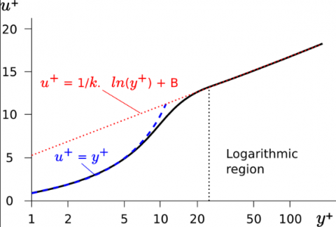
Relationships between velocity and distance from the wall have been established for these regions Figure 2:
Figure 2. Dimensionless velocity profile
$\text { Sublayer laminar : } \mathrm{u}^{+}=y^{+}$ (10)
$\text { Logarithmic sublayer } u^{+}=\frac{1}{0.41} \log \left(y^{+}\right)+5$ (11)
The approximate limits of the layers presented are:
In a turbulent flow, any property (φ fluctuates in time around its mean and can be defined as the sum of the mean value and the fluctuation.
$\varphi=\bar{\varphi}+\dot{\varphi}$ (12)
By replacing, in the continuity and momentum conservation equations for the laminar regime, the variables φ defined by Eq. (12), the mean of the fluctuations is zero, but the mean of the squares of the fluctuations and the products of these fluctuations is not zero.
The equations obtained are similar to the momentum conservation equations for the laminar regime, with the exception of six additional terms, which are called "Reynolds shear stresses":
$-\rho \cdot \overline{u^{\prime 2}},-\rho \cdot \overline{v^{\prime 2}},-\rho \cdot \overline{w^{\prime 2}},-\rho \cdot \overline{u^{\prime} \cdot v^{\prime}},-\rho \cdot \overline{u^{\prime} \cdot w^{\prime}},-\rho \cdot \overline{v^{\prime} \cdot w^{\prime}}$
If we take stock, the system of governing equations is formed of four equations (the continuity equation and three equations of conservation of momentum) and ten unknowns: $\bar{u}, \bar{v}, \bar{w}, \bar{p}$, and the six Reynolds constraints. This is called "the closure problem". We must therefore find relationships to calculate the six additional terms.
Boussinesq based on dimensional analysis, suggested that the Reynolds stresses are calculated with relations similar to those used for the shear stresses in laminar regime, to form:
$-\rho \cdot \overline{u_{l}^{\prime} \cdot u_{j}^{\prime}}=\mu_{t} \cdot\left(\frac{\partial \overline{u_{\imath}}}{\partial x_{j}}+\frac{\partial \bar{u}_{j}}{\partial x_{i}}\right)$ (13)
The eddy viscosity µt ("eddy viscosity") is a scalar, a proportionality constant between the Reynolds shear stresses and the strain rate. Relative to the dynamic molecular viscosity µ, which is a physical property of the fluid and can be measured, the turbulent viscosity µt is a property of a flow and must be modeled. It depends on the flow conditions and varies with the position in the fluid.
The Boussinesq approximation is used in all RANS models, except the RSM models. By expressing the six unknowns, which form the Reynolds stress tensor using this approximation, the problem is reduced to determining a single unknown, which is the turbulent viscosity.
The system of governing equations thus becomes a system of four equations with five unknowns. To be able to solve it, it is necessary to determine µt. Depending on the RANS turbulence model chosen, the turbulent viscosity is expressed as a function of one or more other parameters, which can be:
Turbulence models can be grouped into two categories, depending on how turbulent quantities are calculated: direct numerical simulations (DNS) and RANS (Reynolds Averaged Navier-Stokes Equations) models.
DNS approaches are models for simulating turbulent flows in time and space directly. They represent the most precise simulation methods: the Navier-Stokes equations are solved without approximating the turbulent quantities by a sum between the time average and fluctuations. In fact, by direct simulation any approximation is avoided, except for the numerical discretization of the flow domain, the errors of which can be estimated and calculated. We thus obtain all the possible details of the flow, in time and space. The results obtained are equivalent to an experiment in a laboratory and, in addition, by a non-intrusive technique Ferziger et al. [11]. The disadvantage of these models is that they require enormous computing power, inaccessible, especially for large and complicated geometries. For this reason, hybrid models Figure 3 (combinations between DNS and RANS methods) have been developed, for example the LES (Large Eddy Simulation), or DES (Detached Eddy Simulation) models. They represent a compromise - are less precise than DNS, but more precise than RANS models.
Figure 3. Turbulent models approaches
The RANS approaches consist of solving the governing equations in terms of mean variables and by modeling the turbulent quantities. Depending on the degree of approximation of these quantities, there are algebraic models, models with one equation, for example Spalart-Allmaras), models with two equations (for example k-ε, k-ω, etc.), four-equation models (v2-f), seven-equation models (RSM - Reynolds Stress Models). They have the advantage of being more economical from the point of view of computing resources, but less precise than the DNS, because all of them have certain terms modeled (approximated). To illustrate, we mention that the number of domain computation nodes should be proportional to Re (9/4) Salat et al. [12], and the number of time steps is proportional to Re (3/4) Pope. For a Reynolds number of 2000.
In a turbulent flow, local velocities, temperature, pressure (and local density in the case of compressible fluids) undergo fluctuations in time around their mean values. Thereafter, the vortices appear and disappear and at each instant of time, the structure of the flow is different, but around a medium, stable structure. The idea behind the RANS models is to “capture” this average flow, using a statistical approach. Thus, this fluctuating flow is equivalent (in terms of effects: forces exerted, the amount of heat transferred, pressure losses, etc.) to an average flow where the fluctuations are not "visible", but their effects are felt (forces exerted, the amount of heat transferred, pressure losses, etc.) Trias et al. [13].
In Table 1, the auteur [14] presented an evaluation of computational strategies and their availability for expensive industrial applications in aerodynamics, automotive, and aeronautics. These strategies are based on the validation of the type of flow by the calculation of the Reynolds number (Re), the quality of the mesh chosen for the simulation, and the time necessary for the resolution of the three approaches of the turbulence models (RANS, LES, and DNS).
Table 1. Evaluation of computational strategies and their availability for expensive industrial applications (aerodynamic, automotive and aeronautic type). According to Spalart [14]
|
Approche |
Dependence in Re |
Mesh |
the step of time |
|
RANS |
low |
107 |
103 |
|
LES |
low |
1011.5 |
106.5 |
|
DNS |
strong |
1016 |
107.7 |
In steady state, the average quantities are obtained by considering the time average over a sufficiently wide time interval. In transient conditions, we must call the overall average, which is in fact an arithmetic average of the values of the respective quantity (for a certain moment of time) obtained by repeating the same experiment under similar conditions.
This approximation can provide adequate and sufficient information on turbulent flows, avoiding predicting the effects of each and all eddies. For industrial applications and, in some cases, for research, the average quantities supplied by the RANS models are satisfactory.
In the case of the RSM model, there is an equation for each Reynolds shear stress. However, in these equations, certain terms are modeled.
In general, all RANS models "suffer" from several problems, because the modeling of certain terms calls for calculation "artifices" and unrealistic hypotheses, for example the isotropy of turbulent viscosity.
In the particular case of the k-ε and RSM models, the turbulence equations are valid just in the turbulent nucleus. They are not valid and cannot be integrated into the walls without special treatment. In this region, the system of governing differential equations becomes numerically unstable because several terms of the equations tend towards zero, but at different rates of decrease, Finnie [15]. This problem can be treated in two different ways: either by using models of low Reynolds number (Low-Re models), or of functions of a wall (Wall functions).
Low-Re models use-damping functions to attenuate certain terms in the equations of k and ε whose behavior does not coincide with that theory. That is to say, we compare the exact and modeled equations and we help certain terms of the modeled equations to behave as in the exact equations. Some authors, for example Ciofalo [16], found that they were not able to predict the flow parameters in the complex geometry of narrow and wavy channels and have the disadvantage of requiring many computing resources and being unstable in the convergence.
The functions wall, represent a collection of semi-empirical laws for the unknowns of the system of governing equations of the studied problem: the average velocities, the temperature in the case of a problem with heat transfer and for the turbulent quantities (for example k and ε). These laws are based on the theory of the boundary layer. In fact, by this method, the equations for flow, for heat transfer and for turbulence are integrated up to a distance y=yp (the point P is in the logarithmic sublayer) with respect to the wall. Regions of low Reynolds number 0 < y < yp (the laminar and buffer sublayers) are not part of the computational domain. To find the values of the variables in point P, we assume profiles for these variables, for example a logarithmic correlation for velocities.
If one uses the functions of a wall, the mesh cannot be refined randomly close to the walls, the centroids of the meshes must be located in the logarithmic sublayer (30<y+<300). Standard functions lead to acceptable results for a large number of problems, but they are not recommended under certain flow conditions, which depart from the assumptions made during the development of the model, namely: strong pressure gradients or opposite to the flow, if there is dissemination and attachment of the boundary layer, complex three-dimensional flows (for example rotational), turbulent flows with low Reynolds number, etc.
Besides the "standard wall functions", there are several types of wall functions such as non-equilibrium wall functions (NEWF) and improved wall treatment (enhanced wall).
NEWF have been designed to improve the results of standard functions, which do not give good results for the phenomena just mentioned. Their use leads to improvements, particularly in terms of the coefficient of friction and the Nusselt number for complex flows.
EWT represents a more complex method, which involves the use of a two-zone turbulence model and the application of improved wall functions. Thus, the area of calculation is divided into two areas: an area affected by viscosity (near the wall) and another area - the turbulent core. The separation in two zones can be based on the local Re number or on the y+. This separation is adaptive and dynamic: that is to say the size and the shape of the regions change (adapts) for each problem and, for the same problem, during the iterations, according to the flow conditions.
Two turbulence models will be used: for example, in the case of the use of the k-ε model, the complete k-ε model will be used for the external turbulent region and a simplified model (typically a model with only one equation) in the region near the wall. The improved wall functions consist of the gradual fusion (as a function of the distance from the wall) between the laws for the laminar and logarithmic sub layers (Eqns. (10) and (11)).
The expression of the law is in fact a sum of two terms weighted according to the distance, one for laminar and one turbulent term. This wall treatment has been designed for complicated geometries where the thickness of the boundary layer varies considerably and it can be applied for any mesh: fine (y+ < 1 ... 5), coarse (30 < y+ < 300). It must also not give excessive errors for low quality meshes (too coarse and intermediate (5 < y+ < 30)). It is recommended for flows with a low Reynolds number and / or which involve complex phenomena near the walls.
Figure 4. Velocity profile simulated by different RANS approach
Figure 5. Temperature profile simulated by different RANS approach
Figure 6. Velocity field at the levels of the median planes along the axis (X)
Figure 7. Velocity field at the levels of the median planes along the axis (Y)
In Figures 4 and 5, simulations are performed to determine the velocity and temperature profiles in a passive heating system. This simulation provides a good understanding of all the RANS approaches chosen to develop this studied case.
In Figures 6 and 7, the results obtained during 3D simulations. They were made with a heating, condition due to sunshine by modifying Grashof numbers (Grh) between 107 and 1011. The velocity and mean temperature profiles were presented and analyzed. The study of these profiles as a function of the height in the canal has revealed a change in the flow regime. This change in regime is characterized by increased convective transfer. Three zones have been defined along the hot wall: a laminar zone, a transient, and a turbulent zone.
It is at the level of the upper opening and on the hot and cold walls that the speed profiles differ the most and that the 3D effects are most visible Figure 8. The speeds pass through a maximum at the top of the opening superior. Negative velocities characterizing an entry of fresh air through the lower opening, the speeds are mostly negative in the base opening and positive in the upper opening. This means that there is simultaneously a flow of cool air entering the enclosure from below and a flow of warm air exiting from the top, so this is the case with passive heating by the thermocirculation.
Turbulent flows are significantly influenced by the presence of the walls. In areas very close to the walls, the effects of viscosity reduce fluctuations in tangential velocities. Outside the near-wall, turbulence appears more quickly by producing turbulent kinetic energy due to the mean velocity gradient.
The modeling of near-wall zones has a significant impact on the results of the numerical simulation because the presence of the walls constitutes the main source of vorticity and turbulence and the variability of the turbulent flow shows a strong gradient. The turbulence models defined previously remain valid for the calculation of turbulent flows far from the walls.
Figure 8. Resulting velocity at the level of the planes at the midpoints
This presentation allowed us to draw the following conclusions:
Mixed length models have the advantage of their simplicity, but setting the length to be used is delicate; therefore, the use of this type of model is limited to certain very specific fields of application. The model with two equations k-ε is widely used in industrial applications. Its field of application is wide, and if it suffers from certain limitations, they are however well known. The models of transport of the Reynolds tensions constitutes a means of overcoming the deficiencies of the model k - ε for certain types of flows. However, their use has not really become widespread, perhaps because many commercial codes do not offer sufficiently robust diagrams to use them simply. The near-wall modeling is still relatively rudimentary, and in any case is not yet sufficiently general for the conventional “logarithmic” wall law approaches to be clearly exceeded; this remark is particularly valid for thermal aspects.
LES simulations have appeared in industrial applications for a few years, but they still suffer from a certain lack of maturity of codes and insufficient computing and processing powers. Furthermore, as we expect to see fluctuations appear in such simulations, it is imperative that users have the experience required to differentiate between “physical” fluctuations and purely numerical oscillations, which may arise from insufficient stability of the numerical schemes. Still in the LES, the treatment of near-wall areas, the coupling with other models (RANS, LES) and the consideration of thermal aspects are research fields still widely open.
The DNS remains a tool allowing the study of elementary phenomena with low Reynolds number (for example for the development of models). For all areas, the aspects relating to the calculation uncertainties must be the subject of specific work (numerical, physical uncertainties, confidence interval, etc.).
[1] Xin, S., Le Quéré, P. (1995). Direct numerical simulations of two-dimensional chaotic natural convection in a differentially heated cavity of aspect ratio 4. Journal of Fluid Mechanics, 304: 87-118. https://doi.org/10.1017/s0022112095004356
[2] Tian, Y.S., Karayiannis, T.G. (2000). Low turbulence natural convection in an air filled square cavity: Part I: the thermal and fluid flow fields. International Journal of Heat and Mass Transfer, 43(6): 849-866. https://doi.org/10.1016/s0017-9310(99)00200-8
[3] Peng, S.H., Davidson, L. (2001). Large eddy simulation for turbulent buoyant flow in a confined cavity. International Journal of Heat and Fluid Flow, 22(3): 323-331. https://doi.org/10.1016/s0142-727x(01)00095-9
[4] Sergent, A., Joubert, P., Quéré, P.L. (2003). Development of a local subgrid diffusivity model for large-eddy simulation of buoyancy-driven flows: Application to a square differentially heated cavity. Numerical Heat Transfer: Part A: Applications, 44(8): 789-810. https://doi.org/10.1080/716100524
[5] Ezzouhri, R., Joubert, P., Penot, F., Mergui, S. (2009). Large Eddy simulation of turbulent mixed convection in a 3D ventilated cavity: Comparison with existing data. International Journal of Thermal Sciences, 48(11): 2017-2024. https://doi.org/10.1016/j.ijthermalsci.2009.03.017
[6] Hami, K., Draoui, B., Imine, O., Hami, O. (2016). Thermal fluid modeling of a passive heating system. Journal of Renewable and Sustainable Energy, 8(1): 013113. https://doi.org/10.1063/1.4942542
[7] Hami, K., Draoui, B. (2017). Approche numérique d’un écoulement d’air transitoire (laminaire/turbulent) dans un système de chauffage passif de façade. International Congress on Energetic and Environmental Systems (IEES-2017), Djerba, Tunisie, pp. 1-6.
[8] Zeng, X.P., Wang, Y.S., MacCall, B.T. (2019). A k–e turbulence model for the stable atmosphere. Journal of the Atmospheric Sciences, 77(3): 167-184. https://doi.org/10.1175/JAS-D-19-0085.1
[9] Rodi, W. (2017). Turbulent modeling and simulation in hydraulics: A historical review. Journal of Hydraulic Engineering, 143(5). https://doi.org/10.1061/(ASCE)HY.1943-7900.0001288
[10] Mohammed, K., Sleiti, A.K. (2020). Turbulence modeling using z-f model and RSM for flow analysis in Z-SHAPE ducts. Hindawi, Journal of Engineering. https://doi.org/10.1155/2020/4854837
[11] Ferziger, J.H., Perić, M., Street, R.L. (2002). Computational methods for fluid dynamics. Berlin: Springer, 3: 196-200. https://doi.org/10.1007/978-3-642-56026-2
[12] Salat, J., Xin, S., Joubert, P., Sergent, A., Penot, F., Le Quere, P. (2004). Experimental and numerical investigation of turbulent natural convection in a large air-filled cavity. International Journal of Heat and Fluid Flow, 25(5): 824-832. https://doi.org/10.1016/j.ijheatfluidflow.2004.04.003
[13] Trias, F.X., Gorobets, A., Soria, M., Oliva, A. (2010). Direct numerical simulation of a differentially heated cavity of aspect ratio 4 with Rayleigh numbers up to 1011–Part I: Numerical methods and time-averaged flow. International Journal of Heat and Mass Transfer, 53(4): 665-673. https://doi.org/10.1016/j.ijheatmasstransfer.2009.10.026
[14] Spalart, P.R. (1999). Strategies for turbulence modelling and simulations. In Proc. Fourth Intl Symp. Eng. Turb. Modelling and Measurements, Ajaccio, Corsica, France.
[15] Finnie, J.I. (1994). Introduction to Turbulence Models in: Chaudhry M.H., Mays L.W. (eds) Computer Modeling of Free-Surface and Pressurized Flows, NATO ASI Series (Series E: Applied Sciences), Springer, Dordrecht, 274: 205-239. https://doi.org/10.1007/978-94-011-0964-2_8
[16] Ciofalo, M. (1997). Flow and heat transfer predictions in flow passages of air preheaters: assessment of alternative modeling approaches in Computer simulations in Compact Heat Exchangers, Computational Mechanics Publications, London, UK, pp. 169-225.