Yan Wang | Zhongshui Man* | Meihua Lu
© 2020 IIETA. This article is published by IIETA and is licensed under the CC BY 4.0 license (http://creativecommons.org/licenses/by/4.0/).
OPEN ACCESS
The productivity of coalbed methane (CBM) depends heavily on the heat environment, and directly reflects the quality of the well. Following the theories of phase space reconstruction and Bayesian evidence framework, this paper puts forward a Bayes-least squares-support vector machine (Bayes-LS-SVM) model for the prediction of energy-efficient productivity of CBM under Bayesian evidence network based on chaotic time series. The energy-efficient productivity stands for the gas and water production of CBM wells at a low energy consumption, despite the disturbance from the heat environment. The proposed model avoids the local optimum trap of backpropagation neural network (BPNN), and overcomes the main defects of the SVM: high time consumption of parameter determination, and proneness to overfitting. In our model, the model parameters are optimized through three-layer Bayesian evidence inference, and the input vector for prediction is selected adaptively. In this way, the model construction is not too empirical, and the constructed model is highly adaptive. Then, the theory on phase space reconstruction was applied to investigate the chaotic property of the time series on CBM production, and the Bayes-LS-SVM was adopted to predict the time series after phase space reconstruction, in comparison with neural network prediction methods like SVM and BPNN. Experimental results show that the proposed model boast quick computing, accurate fitting, flexible structure, and strong generalization ability.
chaotic time series, phase space reconstruction, Bayes-least squares-support vector machine (Bayes-LS-SVM), energy-efficient productivity of coalbed methane (CBM)
Energy-efficient productivity stands for the gas and water production of coalbed methane (CBM) wells at a low energy consumption, despite the disturbance from the heat environment. It is an important indicator of the quality of a CBM well. To develop CBM field with a high energy efficiency, it is an urgent issue to predict Energy-efficient CBM productivity accurately. The mining of CBM is an extremely complex system. The gas and water productions of a CBM well are affected by multiple factors, which are sometimes hard to observe or obtain. This severely limits the application of reservoir simulation technology. As a result, it is highly practical to build an effective energy-efficient CBM productivity prediction model that facilitates CBM exploration and development.
In the field of energy-efficient CBM productivity prediction, one of the hot topics is to set up a mathematical prediction model after establishing the nonlinear functional relationship between input and output data through intelligent calculation [1, 2]. Based on modern theories of mathematical statistics, Yang and Qin [3] introduced grey system and time series analysis into energy-efficient CBM productivity prediction, and created a stochastic dynamic prediction model for energy-efficient CBM productivity. Application examples proved that the stochastic dynamic model offers a novel and effective way to predict energy-efficient CBM productivity. Jiang et al. [4], Wu et al. [5] integrated the merits of fuzzy comprehensive evaluation (FCE) and backpropagation neural network (BPNN); the former was adopted to construct the input matrix of the neural network, and the latter was employed to predict the productivity of the gas well. Drawing on modern theories on artificial intelligence and mathematical statistics, Lyu et al. [6] established a time series BPNN model and a monthly production-cumulative production ratio model for fitting and predicting the dynamic productivity of CBM wells, and proved the effectiveness of these models in the fitting and prediction of CBM well productivity.
Based on chaotic time series, this paper proposes an energy-efficient CBM productivity prediction model and its algorithm, that is, the least squares-support vector machine (LS-SVM) under the Bayesian evidence framework. Compared with the traditional learning method of neural network, the LS-SVM has multiple advantages, namely, minimizing structural risk, approximating the global optimum of any function, and fast solving speed. However, the SVM model takes a long time to determine model parameters, and faces a high risk of over-fitting. To optimize the parameters, improve efficiency, and guarantee fitting accuracy, this paper searches for the optimal parameters of the SVM model through the three-layer Bayesian evidence inference. The LS-SVM under the Bayesian framework (Bayes-LS-SVM) could achieve accurate prediction in a timely manner. Experimental results show that the proposed Bayes-LS-SVM model boast quick computing, accurate fitting, flexible structure, and strong generalization ability, opening a new way to predict energy-efficient CBM productivity.
In the 1980s, Packard, Lekscha and Donner [7], Jokar et al., [8] proposed the phase space reconstruction theory, which defines the phase space as a geometric space that determines the phase, i.e., the state of a system at a certain time. The main idea of this theory is as follows: In a dynamic system, the change of any component depends on its closely related components. Instead of being isolated, every component in the system contains the evolution information of other components. The phase space reconstruction of time series is grounded on the fact that, a univariate time series comprehensively reflects the interaction between many physical factors, and carries the traces of all variables. To fully reveal the embedded information, the time series should be expanded to the three-dimensional or higher-dimensional phase space [9, 10].
Let x={xi=1,2,…,N} be the time series of a component in a system. Then, the state vector reconstructed at a point in the phase space can be expressed as:
$X=\left\{ \begin{align} & {{X}_{i}}\mid {{X}_{i}}={{\left[ {{x}_{i}},{{x}_{i+t}},\ldots ,{{x}_{i+(m-1)t}} \right]}^{T}}, \\ & i=1,2,\ldots ,M \\\end{align} \right\}$ (1)
where, M=N-(m-1)t is the number of points in the reconstructed phase space; m and t are the embedding dimension and time delay of the system, respectively. Takens highlighted the importance of determining the values of m and t. There are two opposite views on the selection of the two parameters: Some scholars held that the two parameters are not correlated, i.e., m and t need to be selected independently; some believed that m is correlated with t, i.e., the selections of m and t are mutually dependent, and the two parameters could be calculated simultaneously by time window method or C-C method. Here, the C-C method is selected to determine the m and t values [11, 12].
3.1 LS-SVM
Facing large sample data, the SVM often consume a long time and take up a huge memory. To solve these defects, Sun et al. [13], Tan et al. [14], Suykens and Vandewalle [15] put forward an LS-SVM under equation constraints, using the sum of squares for error (SSE) as the loss function. The LS-SVM not only reduces the number of undetermined parameters in the SVM model, but also lowers the difficulty in parameter selection [16-18].
According to the structural risk minimization criterion, the LS-SVM model for solving the regression function can be described by:
$\min \frac{1}{2}{{\left\| w \right\|}^{2}}+\frac{1}{2}\gamma \sum\limits_{i=1}^{n}{\xi _{i}^{2}}$
$s.t.\text{ }{{y}_{i}}-{{w}^{T}}\varphi ({{x}_{i}})-b={{e}_{i}},\left( i=1,2,...,n \right)$
In the optimization problem, the LS-SVM adopts the following Lagrange function:where, ei is the error between the true value and predicted value; γ>0 is the penalty coefficient.
$\begin{align} & L\left( \omega ,b,\xi ,\alpha \right)=\frac{1}{2}{{\left\| w \right\|}^{2}}+\frac{1}{2}\gamma \sum\limits_{i=1}^{n}{e_{i}^{2}} \\ & +\sum\limits_{i=1}^{n}{{{\alpha }_{i}}}\left[ {{w}^{T}}\varphi ({{x}_{i}})+b+{{e}_{i}}-{{y}_{i}} \right] \\\end{align}$ (3)
where, αi is the Lagrangian multiplier.
Finding the partial derivatives of αi, b, ei, and w in formula (3), the optimality conditions can be expressed as:
$\left\{ \begin{align} & \frac{\partial L}{\partial w}=0\to w=\sum\limits_{i=1}^{n}{{{\alpha }_{i}}\varphi \left( {{x}_{i}} \right)} \\ & \frac{\partial L}{\partial b}=0\to \sum\limits_{i=1}^{n}{{{\alpha }_{i}}=0,i=1,...n} \\ & \frac{\partial L}{\partial {{e}_{i}}}=0\to {{\alpha }_{i}}=\gamma {{e}_{i}},i=1,...n \\ & \frac{\partial L}{\partial {{\alpha }_{i}}}=0\to {{w}^{T}}\varphi ({{x}_{i}})+b+{{e}_{i}}-{{y}_{i}}=0,i=1,...n \\\end{align} \right.$ (4)
Simplifying formula (4):
${{\left[ \begin{matrix} 0 & 1_{n}^{T} \\ {{1}_{n}} & Z{{Z}^{T}}+{}^{I}/{}_{\gamma } \\\end{matrix} \right]}_{\left( n+1 \right)\times \left( n+1 \right)}}\left[ \begin{matrix} \begin{matrix} b \\ \alpha \\\end{matrix} \\\end{matrix} \right]=\left[ \begin{align} & 0 \\ & y \\\end{align} \right]$ (5)
where, $Z=\left[\varphi\left(x_{1}\right), \varphi\left(x_{2}\right), \ldots \varphi\left(x_{n}\right)\right]^{T} ; y=\left[y_{1}, y_{2}, \ldots y_{n}\right]^{T}$; $1_{n}=[1,1 \ldots 1]^{T} ; \alpha=\left[\alpha_{1}, \alpha_{2}, \ldots \alpha_{n}\right]^{T}$; I is an n´n-order unit matrix. The kernel function can be defined as:
$K\left( {{x}_{i}},{{x}_{j}} \right)=\varphi {{\left( {{x}_{i}} \right)}^{T}}\varphi \left( {{x}_{j}} \right)$ (6)
Formula (5) can be rewritten as:
$\left[\begin{array}{cccc}
0 & 1 & \ldots & 1 \\
1 & K\left(x_{1}, x_{1}\right)+\frac{1}{\gamma} & \ldots & K\left(x_{1}, x_{l}\right) \\
\vdots & \vdots & \vdots & \vdots \\
1 & K\left(x_{l}, x_{1}\right) & \ldots & K\left(x_{l}, x_{l}\right)+\frac{1}{\gamma}
\end{array}\right]\left[\begin{array}{l}
b \\
\alpha_{1} \\
\vdots \\
\alpha_{l}
\end{array}\right]=\left[\begin{array}{l}
0 \\
y_{1} \\
\vdots \\
y_{l}
\end{array}\right]$ (7)
The values of a and b can be found by solving formula (7). Thus, the prediction function of the LS-SVM can be expressed as:
$f\left( x \right)=\sum\limits_{i=1}^{n}{{{\alpha }_{i}}}K\left( {{x}_{i}},x \right)+b$ (8)
3.2 Bayesian evidence framework
Since its proposal by MacKay, the Bayesian evidence framework has been widely applied in neural networks. The main idea of this framework is to maximize the posterior of parameter distribution [19, 20]. Generally, the Bayesian evidence framework can be divided into three inference criteria. Let H be a model; λ be a regularized parameter; w be a k-dimensional parameter vector of the model. Then, the prior distribution of w can usually be expressed as [21-24]:
$P(w|\lambda ,H)=\frac{\exp \left( -\lambda {{E}_{w}}\left( w|H \right) \right)}{{{Z}_{w}}\left( \lambda \right)}$ (9)
where,
$\begin{align} & {{Z}_{w}}\left( \lambda \right)=\int{\exp \left( -\lambda {{E}_{w}}\left( w|H \right){{d}^{k}}w \right)}, \\ & {{E}_{w}}={{w}^{T}}{w}/{2}\; \\\end{align}$ (10)
3.2.1 Inference criterion 1
Under this criterion, the posterior of w is inferred by the Bayes rule. Let D be a dataset. Then, the following can be derived from the Bayes formula:
$P(w|D,\lambda ,H)\infty P(D|w,H)P(w|\lambda ,H)$ (11)
Substituting formula (9) into formula (12), we have $P(w \mid D, \lambda, H)=P(D \mid w, H)$;
$\begin{align} & \frac{\exp \left( -\lambda {{E}_{w}}\left( w|H \right) \right)}{\int{P(D|w,H)\exp \left( -\lambda {{E}_{w}}\left( w|H \right) \right){{d}^{k}}w}} \\ & =\frac{\exp \left( -M\left( w \right) \right)}{{{Z}_{M}}\left( \lambda \right)} \\\end{align}$ (12)
Thus, $M(w)=\lambda E_{w}(w \mid H)-\ln P(D \mid w, H)$; $Z_{M}(\lambda)=\int \exp (-M(w)) d^{k} w$.
3.2.2 Inference criterion 2
Based on the posterior of λ, the posterior of w is approximated by Gaussian distribution:
$\begin{align} & P(w|D,\lambda ,H)\cong \\ & \frac{\exp \left( -M\left( {{\omega }_{MP}} \right)-{1}/{2{{\left( \omega -{{\omega }_{MP}} \right)}^{'}}A\left( \omega -{{\omega }_{MP}} \right)}\; \right)}{Z_{M}^{\text{ }\!\!'\!\!\text{ }}} \\\end{align}$ (13)
where, $A=\nabla^{2} M$ is a Hessian matrix. The evidence λ can be obtained by integrating w:
$\begin{align} & \ln P(D|\lambda ,H)=-\lambda E_{W}^{MP}+ \\ & \ln P(D|w,H)\left| w={{w}_{MP}}-\frac{1}{2} \right.\ln \det A+\frac{k}{2}\ln \lambda \\\end{align}$ (14)
To obtain λMP, the partial derivative of formula (14) relative to λ needs to be set as zero. Then, we have:
$2{{\lambda }_{MP}}E_{W}^{MP}=\gamma $ (15)
where, $\gamma=k-\lambda \operatorname{trace} A^{-1}$ is the significance of a parameter.
3.2.3 Inference criterion 3
Criterion 3 derives the optimal kernel parameters by evaluating the pros and cons of different models based on posterior probability. According to the Bayes formula, $P(H \mid D)$$\infty$$P(D \mid H) P(H)$. Suppose P(H) obeys a flat distribution. Then, P(D|H) satisfies:
$P(D|H)=\int{P(D|\lambda ,H)}P(\lambda |H)d\lambda $ (16)
Through Gaussian approximation of $P(D \mid \lambda, H)$, we have:
$P(D|H)\infty {P(D|{{\lambda }_{MP}},H)}/{\sqrt{\gamma }}\;$ (17)
In this paper, the LS-SVM improved under the Bayesian evidence framework, that is, the Bayes-LS-SVM, is applied to predict energy-efficient CBM productivity, and proved feasible and effective in comparison with BPNN and SVM.
4.1 Evaluation metrics
The model accuracy in energy-efficient CBM productivity prediction was mainly measured by root mean square error (RMSE) and mean squared error (MSE):
$RMSE=\sqrt{\frac{\sum\limits_{i=1}^{n}{{{\left( {{{\hat{x}}}_{i,n}}-{{x}_{i,n}} \right)}^{2}}}}{N{{\sigma }^{2}}}}$ (18)
where, $x_{i, n} \text { and } \hat{x}_{i, n}$ are the true value and predicted value, respectively; σ2 is the variance; N is the length of the time series.
$MAE=\frac{1}{N}\sum\limits_{i=1}^{n}{\left| {{{\hat{x}}}_{i,n}}-{{x}_{i,n}} \right|}$ (19)
where, N is the total number of predictions [25-27].
The RMSE characterizes the degree of dispersion of samples. The more accurate the predicted value, the smaller the RMSE. The MSE adopts the absolute value of the degree of dispersion, so that positive and negative values no longer cancel each other. Hence, the MSE provides a more realistic depiction of prediction error than the mean error.
4.2 Application verification
The CBM production from December 1, 2007 to September 21, 2008 and the water production from December 1, 2007 to March 14, 2008 of CBM well PZ02 in a mining area were taken as the basis for application verification.
4.2.1 Data selection and preprocessing
A total of 300 gas production data and 105 water production data were collected from well PZ02. The first 280 gas production data were treated as training samples, and the last 20 as prediction samples. The first 85 water production data were treated as training samples, and the last 20 as prediction samples. The selected data carry significant nonlinearity.
To meet the requirements of relevant functions of the prediction model, the extreme value method was selected to normalize the collected data. This method does not have any specific requirement on the distribution and number of data, or other aspect of data information. After normalization by this method, the input data were converted into the interval of [0, 1].
4.2.2 Judgment of chaotic property of time series and phase space reconstruction
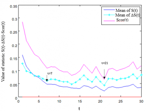
First, the training samples of gas production data were subject to phase space reconstruction and the judgement of the chaotic property of time series. By C-C algorithm, the embedding dimension m was determined as 4, and the optimal delay was derived as t=7 (unit: day) (Figure 1(a)).
The chaotic property of the time series of gas production was judged by the Lyapunov exponent. Here, the maximum Lyapunov exponent is calculated by Wolf’s algorithm. To maximize the Lyapunov exponent, Wolf et al. identified the evolution point (predicted value) of the current point (the center point) by limiting both the distance and angle between the two points, such that the evolution point must fall on the track adjacent to the current point. When Lyapunov exponent is selected for prediction, the angle should be limited to ensure that the evolution point falls on the track adjacent to the current point. Through calculation, the maximum Lyapunov exponent was obtained as λ=0.047. Since the exponent is greater than zero, the historical data on gas production are chaotic.
(a)
(b)
Figure 1. The relationship between embedding dimension and time delay in gas production (a) and water production (b)
In Figure 1(a), the first minimum of DS appeared at t=7, indicating that the optimal delay tau=7. The global minimum of Scor was observed at t=21, suggesting that tw=21. Since tw=(m-1), it could be obtained that the embedding dimension m=4.
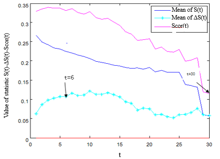
Next, the phase space reconstruction and the judgement of the chaotic property were performed on the water production training samples. By C-C algorithm, the embedding dimension m was determined as 6, and the optimal delay was derived as t=6 (Figure 1(b)). Lyapunov exponent is the key indicator of whether the time series of water output is chaotic. The maximum Lyapunov exponent was derived by Wolf’s algorithm as λ=0.023. Since the exponent is greater than zero, the historical data on water production are chaotic.
4.2.3 Training and prediction
Based on the selected initial parameters, the Bayes-LS-SVM model was trained by the training samples of gas and water productions of the CBM well. The radial basis kernel function was chosen, owing to its better performance over other kennel functions. The regression model was trained in three steps: the optimal parameters b and w were inferred on the first layer of the Bayesian framework; the regularization parameter γ was inferred on the second layer; the optimal kernel parameter σ was inferred on the third layer. Through trial and error, the optimal parameters of the energy-efficient CBM productivity prediction model were obtained as the γ and σ making the p(D|H) value reach the maximum.
Repeated calculations show that, for the gas production training samples, the optimal kernel parameter was σ=148.41, and the optimal regularization parameter was γ=203.78; for the water production training samples, the optimal kernel parameter was σ=185.74, and the optimal regularization parameter was γ=1.6456. Finally, the trained model was applied to predict the test samples, and de-normalize the predicted data. The final predicted values are compared with the true values in Tables 1 and 2. The prediction curves are recorded in Figure 2.
Table 1. The true and predicted gas productions of the CBM well m3/d
|
Serial number |
True value |
Predicted value |
Relative error % |
Serial number |
True value |
Predicted value |
Relative error % |
|
1 |
1300 |
1264.71 |
2.71462 |
11 |
913 |
937.16 |
2.646221 |
|
2 |
1155 |
1130.82 |
2.09351 |
12 |
880 |
886.76 |
0.768182 |
|
3 |
950 |
997.78 |
5.029474 |
13 |
750 |
769.59 |
2.612 |
|
4 |
1020 |
997.78 |
2.17843 |
14 |
750 |
776.93 |
3.590667 |
|
5 |
900 |
904.40 |
0.488889 |
15 |
930 |
919.90 |
1.08602 |
|
6 |
800 |
822.28 |
2.785 |
16 |
1000 |
969.05 |
3.095 |
|
7 |
860 |
895.36 |
4.111628 |
17 |
1000 |
967.94 |
3.206 |
|
8 |
900 |
923.39 |
2.598889 |
18 |
1200 |
1095.89 |
8.67583 |
|
9 |
920 |
930.75 |
1.168478 |
19 |
1065 |
1056.92 |
0.75869 |
|
10 |
894 |
912.55 |
2.074944 |
20 |
1100 |
1078.95 |
1.91364 |
Table 2. The true and predicted water productions of the CBM well m3/d
|
Serial number |
True value |
Predicted value |
Relative error % |
Serial number |
True value |
Predicted value |
Relative error % |
|
1 |
0.40 |
0.4150 |
3.75 |
11 |
0.20 |
0.2001 |
0.05 |
|
2 |
0.60 |
0.6037 |
0.616667 |
12 |
0.40 |
0.3740 |
6.5 |
|
3 |
0.50 |
0.5168 |
3.36 |
13 |
0.50 |
0.4694 |
6.12 |
|
4 |
0.40 |
0.4018 |
0.45 |
14 |
0.30 |
0.3138 |
4.6 |
|
5 |
0.60 |
0.5874 |
2.1 |
15 |
0.20 |
0.2069 |
3.45 |
|
6 |
0.50 |
0.4999 |
0.02 |
16 |
0.30 |
0.2913 |
2.9 |
|
7 |
0.30 |
0.3128 |
4.266667 |
17 |
0.50 |
0.4914 |
1.72 |
|
8 |
0.20 |
0.2026 |
1.3 |
18 |
0.70 |
0.7053 |
0.757143 |
|
9 |
0.40 |
0.3805 |
4.875 |
19 |
0.90 |
0.9106 |
1.177778 |
|
10 |
0.30 |
0.313 |
4.333333 |
20 |
0.80 |
0.7611 |
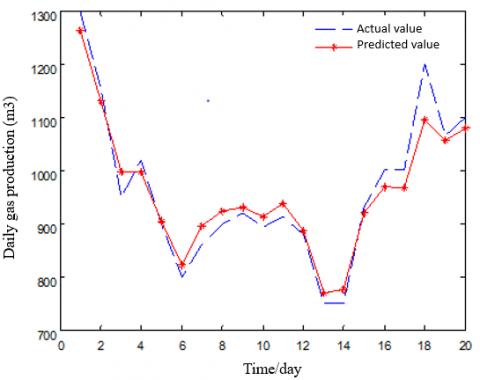
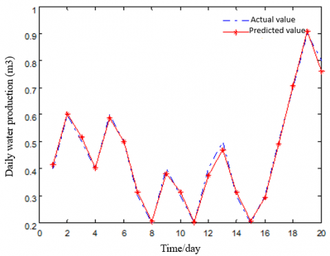
4.8625 |
As shown in Tables 1 and 2, the gas productions predicted by the proposed model were close to the true value of the CBM well. The relative error between predicted and true values was large only for a very few data. Hence, the Bayes-LS-SVM model achieved a good effect. To more intuitively compare predicted and true values, the two values were fitted into the following figure (Figure 2). As shown in Figure 2, the broken lines on the true productivities of the CBM well were almost identical to those on the productivities predicted by the Bayes-LS-SVM, except for very few data points.
(a)
(b)
Figure 2. The fitted predicted and true values of gas production (a) and water production (b)
4.2.4 Comparative analysis
Table 3. The predicted gas productions of the three models
|
Serial number |
Daily gas production (m3) |
BPNN |
SVM |
Bayes-LS-SVM |
|||
|
Predicted value (m3) |
Relative error (%) |
Predicted value (m3) |
Relative error (%) |
Predicted value (m3) |
Relative error (%) |
||
|
1 |
1,300 |
1,194.84 |
8.08923 |
1237.58 |
4.80154 |
1264.71 |
2.71462 |
|
2 |
1,155 |
1,203.28 |
4.180087 |
1182.75 |
2.402597 |
1130.82 |
2.09351 |
|
3 |
950 |
989.04 |
4.109474 |
1016.25 |
6.973684 |
997.78 |
5.029474 |
|
4 |
1,020 |
949.34 |
6.92745 |
990.39 |
2.90294 |
997.78 |
2.17843 |
|
5 |
900 |
933.73 |
3.747778 |
903.73 |
0.414444 |
904.40 |
0.488889 |
|
6 |
800 |
840.07 |
5.00875 |
848.62 |
6.0775 |
822.28 |
2.785 |
|
7 |
860 |
928.68 |
7.986047 |
902.50 |
4.94186 |
895.36 |
4.111628 |
|
8 |
900 |
952.81 |
5.867778 |
933.63 |
3.736667 |
923.39 |
2.598889 |
|
9 |
920 |
970.58 |
5.497826 |
928.31 |
0.903261 |
930.75 |
1.168478 |
|
10 |
894 |
946.13 |
5.831096 |
911.46 |
1.95302 |
912.55 |
2.074944 |
|
11 |
913 |
895.72 |
1.89266 |
967.35 |
5.952903 |
937.16 |
2.646221 |
|
12 |
880 |
925.11 |
5.126136 |
885.69 |
0.646591 |
886.76 |
0.768182 |
|
13 |
750 |
808.99 |
7.865333 |
801.58 |
6.877333 |
769.59 |
2.612 |
|
14 |
750 |
843.75 |
12.5 |
828.73 |
10.49733 |
776.93 |
3.590667 |
|
15 |
930 |
978.84 |
5.251613 |
928.06 |
0.2086 |
919.90 |
1.08602 |
|
16 |
1,000 |
930.75 |
6.925 |
971.36 |
2.864 |
969.05 |
3.095 |
|
17 |
1,000 |
948.62 |
5.138 |
957.17 |
4.283 |
967.94 |
3.206 |
|
18 |
1,200 |
1,098.37 |
8.46917 |
1096.29 |
8.6425 |
1095.89 |
8.67583 |
|
19 |
1,065 |
1,109.24 |
4.153991 |
1032.74 |
3.02911 |
1056.92 |
0.75869 |
|
20 |
1,100 |
1,149.21 |
4.473636 |
1079.49 |
1.86455 |
1078.95 |
1.91364 |
Table 4. The predicted water productions of the three models
|
Serial number |
Daily water production (m3) |
BPNN |
SVM |
Bayes-LS-SVM |
|||
|
Predicted value (m3) |
Relative error (%) |
Predicted value (m3) |
Relative error (%) |
Predicted value (m3) |
Relative error (%) |
||
|
1 |
0.40 |
0.4153 |
3.825 |
0.4176 |
4.4 |
0.4150 |
3.75 |
|
2 |
0.60 |
0.6075 |
1.25 |
0.6018 |
0.3 |
0.6037 |
0.616667 |
|
3 |
0.50 |
0.5324 |
6.48 |
0.5146 |
2.92 |
0.5168 |
3.36 |
|
4 |
0.40 |
0.4232 |
5.8 |
0.4049 |
1.225 |
0.4018 |
0.45 |
|
5 |
0.60 |
0.6221 |
3.683333 |
0.5921 |
1.31667 |
0.5874 |
2.1 |
|
6 |
0.50 |
0.5137 |
2.74 |
0.5109 |
2.18 |
0.4999 |
0.02 |
|
7 |
0.30 |
0.3191 |
6.366667 |
0.3141 |
4.7 |
0.3128 |
4.266667 |
|
8 |
0.20 |
0.2283 |
14.15 |
0.2061 |
3.05 |
0.2026 |
1.3 |
|
9 |
0.40 |
0.4101 |
2.525 |
0.4214 |
5.35 |
0.3805 |
4.875 |
|
10 |
0.30 |
0.3228 |
7.6 |
0.3066 |
2.2 |
0.313 |
4.333333 |
|
11 |
0.20 |
0.2071 |
3.55 |
0.2298 |
14.9 |
0.2001 |
0.05 |
|
12 |
0.40 |
0.4136 |
3.4 |
0.4085 |
2.125 |
0.3740 |
6.5 |
|
13 |
0.50 |
0.4529 |
9.42 |
0.4693 |
6.14 |
0.4694 |
6.12 |
|
14 |
0.30 |
0.3124 |
4.133333 |
0.3149 |
4.966667 |
0.3138 |
4.6 |
|
15 |
0.20 |
0.2473 |
23.65 |
0.2320 |
16 |
0.2069 |
3.45 |
|
16 |
0.30 |
0.3192 |
6.4 |
0.3086 |
2.866667 |
0.2913 |
2.9 |
|
17 |
0.50 |
0.5635 |
12.7 |
0.4923 |
1.54 |
0.4914 |
1.72 |
|
18 |
0.70 |
0.7263 |
3.757143 |
0.608 |
13.1429 |
0.7053 |
0.757143 |
|
19 |
0.90 |
0.8547 |
5.03333 |
0.8876 |
1.37778 |
0.9106 |
1.177778 |
|
20 |
0.80 |
0.7831 |
2.1125 |
0.7857 |
1.7875 |
0.7611 |
4.8625 |
To demonstrate its excellence in prediction, the proposed Bayes-LS-SVM was compared with SVM prediction model and BPNN prediction model. The two contrastive models were trained and tested on the same data as our model, using the same input and output variables.
At present, the BPNN is usually optimized by conjugate gradient algorithm, variable rate algorithm, additional momentum algorithm, Levenberg-Marquardt (LM) algorithm, and Gauss-Newton algorithm. Among them, the LM algorithm has relatively fast convergence and good robustness. Hence, this algorithm was chosen to establish the BPNN model. Meanwhile, the SVM model was set up with standard SVM, which is superior for nonlinear, small sample and high-dimensional pattern recognition. The radial basis kernel function was selected as the kernel function. Tables 3 and 4 present the predicted values and relative errors of the three models.
Comparing the predicted gas productions, the BPNN model had a large relative error between predicted and true values; the SVM model had a relatively small relative error, and better prediction performance than BPNN; the Bayes-LS-SVM model achieved the highest prediction accuracy, for the relative error was very low except for very few predicted values.
From Tables 3 and 4, it can be seen that the Bayes-LS-SVM could predict the productivity of the CBM well more accurately than BPNN and SVM models, an evidence for its advantage in energy-efficient CBM productivity forecast. Further, the MSE and RMSE of the three model were calculated and compared to confirm which is the most suitable method for CBM productivity prediction (Tables 5 and 6).
Table 5. The MSEs and RMSEs of the three models (gas production)
|
Model |
MSE (%) |
RMSE (%) |
|
BPNN |
5.9521 |
6.3571 |
|
SVM |
3.9987 |
4.8646 |
|
Bayes-LS-SVM |
2.6798 |
3.2169 |
Table 6. The MSEs and RMSEs of the three models (water production)
|
Model |
MSE (%) |
RMSE (%) |
|
BPNN |
6.4288 |
8.23 |
|
SVM |
4.6244 |
6.4581 |
|
Bayes-LS-SVM |
2.8605 |
3.4823 |
As shown in Tables 5 and 6, on the prediction of gas production, BPNN, SVM, and Bayes-LS-SVM had an MSE of 5.9521%, 3.9987%, and 2.6798%, respectively, and an RMSE of 6.3571%, 4.8646%, and 3.2169%, respectively; on the prediction of water production, BPNN, SVM, and Bayes-LS-SVM had an MSE of 6.4288%, 4.6244%, and 2.8605%, respectively, and an RMSE of 8.23%, 6.4581%, and 3.4823%, respectively. Obviously, Bayes-LS-SVM achieved lower prediction errors than the SVM and BPNN. It is obviously more suitable for predicting CBM productivity.
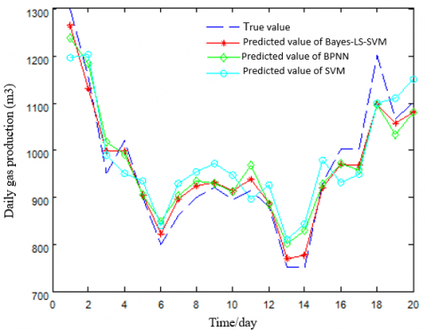
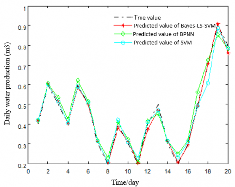
To provide a clear picture of the CBM productivity prediction performance of the three models, the predicted values of these models are compared with the true gas and water productions (Figure 3).
(a)
(b)
Figure 3. The predicted values of the three models on gas production (a) and water production (b)
As shown in Figure 3, the predicted values of Bayes-LS-SVM model agreed well with the true values. The broken lines of the predicted values almost overlapped with those on the true values. Comparatively, the Bayes-LS-SVM model is more suitable for CBM productivity prediction than the other models.
The traditional BPNN model is susceptible to the local optimum trap. Meanwhile, the standard SVM model consumes too much time in parameter determination, and tends to face the over-fitting problem. To overcome these defects, this paper proposes a novel CBM productivity prediction method based on chaotic time series and Bayesian evidence framework, and verifies the performance of the model through experiments. The main conclusions are as follows:
(1) Following the phase space reconstruction theory, the chaotic property of the time series on CBM productivity was discussed, and the C-C method was adopted to compute the time delay t and embedding dimension m.
(2) The model parameters were optimized by three-layer inference of Bayesian evidence framework. The optimization enables the adaptive selection of input variables for prediction, reduces the dependence of model construction on experience, and improves efficiency and fitting accuracy, making the model more adaptive.
(3) The Bayes-LS-SVM was applied to predict the time series after phase space reconstruction, in comparison to BPNN and SVM. The results show that the Bayes-LS-SVM achieved an MSE of only 2.6798%, and an RMSE of merely 3.2169% in the forecast of the gas production in a CBM well, both of which were smaller than those of BPNN and SVM; Bayes-LS-SVM achieved an MSE of only 2.8605%, and an RMSE of merely 3.4823%, in the forecast of the gas production in a CBM well, both of which were smaller than those of BPNN and SVM. The experimental results confirm that the predicted values of Bayes-LS-SVM agree well with the true values, suggesting that our model is suitable for CBM productivity prediction.
This work was supported by National Natural Science Foundation of China (Grant No.: 40972207); National Major Science and Technology Project (Grant No.: 2011ZX05034-005); Doctoral Research Fund (Grant No.: 102081902).
[1] Mei, Y.Y., Qin, Y.Q. (2018). Study on water production of coalbed methane well by using BP neural network. Coal Technology, 37(12): 163-165. https://doi.org/10.13301/j.cnki.ct.2018.12.059
[2] Feng, D.M., Wu, J.W. (2017). Recognition model for mine water inrush sources based on SVM. Journal of Liaoning Technical University (Natural Science Edition), 36(1): 23-27. https://doi.org/10.11956/j.issn.1008-0562.2017.01.004
[3] Yang, Y.G., Qin, Y. (2001). Study and application on random dynamic model of the coalbed methane output forecasting. Journal of China Coal Society, 26(2): 122-125. https://doi.org/10.3321/j.issn:0253-9993.2001.02.003
[4] Jiang, Y.Q., Li, C.Y., Li, Z.J. (2009). New mode of gas well productivity forecast based on fuzzy comprehensive evaluation and BP neural network. Oil-Gasfield Surface Engineering, 28(10): 5-7. https://doi.org/10.3969/j.issn.1006-6896.2009.10.003
[5] Wu, C.F., Yao, S., Du, Y.F. (2015). Production systems optimization of a CBM well based on a time series BP neural network. Journal of China University of Mining & Technology, 44(1): 64-69.
[6] Lyu, Y.M., Tang, D.Z., Li, Z.P., Shao, X.J., Xu, H. (2011). Coalbed methane well dynamic productivity fitting and prediction model. Journal of China Coal Society, 2011(9): 1481-1485.
[7] Lekscha, J., Donner, R.V. (2018). Phase space reconstruction for non-uniformly sampled noisy time series. Chaos: An Interdisciplinary Journal of Nonlinear Science, 28(8): 085702. https://doi.org/10.1063/1.5023860
[8] Jokar, M., Salarieh, H., Alasty, A. (2019). On the existence of proper stochastic Markov models for statistical reconstruction and prediction of chaotic time series. Chaos, Solitons & Fractals, 123: 373-382. https://doi.org/10.1016/j.chaos.2019.04.008
[9] Ong, P., Zainuddin, Z. (2019). Optimizing wavelet neural networks using modified cuckoo search for multi-step ahead chaotic time series prediction. Applied Soft Computing, 80: 374-386. https://doi.org/10.1016/j.asoc.2019.04.016
[10] Monfared, M., Fazeli, M., Lewis, R., Searle, J. (2019). Fuzzy predictor with additive learning for very short-term PV power generation. IEEE Access, 7: 91183-91192. https://doi.org/10.1109/ACCESS.2019.2927804
[11] Takens, F. (1981). Detecting strange attractors in turbulence. In Dynamical Systems and Turbulence, Warwick, 898: 361-381. https://doi.org/10.1007/BFb0091924
[12] Kim, H., Eykholt, R., Salas, J.D. (1999). Nonlinear dynamics, delay times, and embedding windows. Physica D: Nonlinear Phenomena, 127(1-2): 48-60. https://doi.org/10.1016/S0167-2789(98)00240-1
[13] Sun, J.G., Wang, S., Yang, J.X., Xue, R., Pan, H.G. (2018). Single-joint control of closed-loop brain-machine interfaces based on genetic algorithm LS-SVM direct inverse model. Information and Control, 47(6): 656-662. https://doi.org/10.13976/j.cnki.xk.2018.7324
[14] Tan, P.N., Steinbach, M., Kumar, V. (2016). Introduction to Data Mining. Pearson Education India. 2018.
[15] Suykens, J.A., Vandewalle, J. (1999). Least squares support vector machine classifiers. Neural Processing Letters, 9(3): 293-300. https://doi.org/10.1023/A:1018628609742
[16] Shi, X.T., Zhu, B.Z. (2017). Carbon price forecasting based on phase space reconstruction and least square support vector regression. Journal of Systems Science and Mathematical Sciences, 37(2): 562-572.
[17] Paudel, S., Elmitri, M., Couturier, S., Nguyen, P.H., Kamphuis, R., Lacarrière, B., Le Corre, O. (2017). A relevant data selection method for energy consumption prediction of low energy building based on support vector machine. Energy and Buildings, 138: 240-256. https://doi.org/10.1016/j.enbuild.2016.11.009
[18] Zhou, D.P., Wang, Z.W., Li, X.C. (2016). The application of GRNN and LS-SVM to coal properties calculation. Geophysical and Geochemical Exploration, 40(1): 88-92. https://doi.org/10.11720/wtyht.2016.1.16
[19] Huang, J., Malone, B.P., Minasny, B., McBratney, A.B., Triantafilis, J. (2017). Evaluating a Bayesian modelling approach (INLA-SPDE) for environmental mapping. Science of the Total Environment, 609: 621-632. https://doi.org/10.1016/j.scitotenv.2017.07.201
[20] Rue, H., Riebler, A., Sørbye, S.H., Illian, J.B., Simpson, D.P., Lindgren, F.K. (2017). Bayesian computing with INLA: A review. Annual Review of Statistics and Its Application, 4: 395-421. https://doi.org/10.1146/annurev-statistics-060116-054045
[21] Jospin, L.V., Buntine, W., Boussaid, F., Laga, H., Bennamoun, M. (2020). Hands-on Bayesian neural networks-A tutorial for deep learning users. arXiv preprint arXiv:2007.06823. 1(1): 1-35.
[22] Gyamfi, K.S., Brusey, J., Hunt, A., Gaura, E. (2018). Linear dimensionality reduction for classification via a sequential Bayes error minimisation with an application to flow meter diagnostics. Expert Systems with Applications, 91: 252-262. https://doi.org/10.1016/j.eswa.2017.09.010
[23] Peng, Z., Jiang, Y., Yang, X., Zhao, Z., Zhang, L., Wang, Y. (2018). Bus arrival time prediction based on PCA-GA-SVM. Neural Network World, 28(1): 87-104. https://doi.org/10.14311/NNW.2018.28.005
[24] Reddy, K.S.S., Bindu, C.S. (2019). StreamSW: A density-based approach for clustering data streams over sliding windows. Measurement, 144: 14-19. https://doi.org/10.1016/j.measurement.2018.11.041
[25] Fan, G., Sun, R. C., Shao, F.J. (2018). Bus arrival time prediction based on LSTM and Kalman filtering. Computer Applications and Software, 35(4): 91-96.
[26] Ilich, N., Gharib, A., Davies, E.G. (2018). Kernel distributed residual function in a revised multiple order autoregressive model and its applications in hydrology. Hydrological Sciences Journal, 63(12): 1745-1758. https://doi.org/10.1080/02626667.2018.1541090
[27] Kuster, C., Rezgui, Y., Mourshed, M. (2017). Electrical load forecasting models: A critical systematic review. Sustainable Cities and Society, 35: 257-270. https://doi.org/10.1016/j.scs.2017.08.009