Abderrahmane Horimek* | El-Amria Nekag
© 2020 IIETA. This article is published by IIETA and is licensed under the CC BY 4.0 license (http://creativecommons.org/licenses/by/4.0/).
OPEN ACCESS
Cooling process of a heat source placed at the bottom side of a cold-walled cavity (TC) by means of natural convection has been studied numerically in this work. Two thermal conditions have been assumed at the source (q-imposed or T-imposed). The effects of Rayleigh number (Ra=10+3→10+6), source length (SL=0.1→1.0), source position (D) compared to left side, in addition to the effect of the number of Prandtl (Pr=0.71→10+2) were analyzed with ample details. For a source at the center of the bottom side, results showed an increase of flow and temperature disturbance with increasing Ra and/or SL, with an enhancement of both local and mean Nusselt numbers. Particular exceptions were noticed for high Ra values for the second heating type. For all considerations, the case of SL=0.1 makes an exception where a very good heat exchange rate is recorded. When the source is no longer centered, Clearer difference between this case and the previous one was recorded, especially for small D values. Very good heat exchange rate is recorded for D=0.0 for all considerations, with remarkable amount of difference compared the closest one to it, followed by a progressive decrease until the case of source at the center. Finally, Prandtl number (Pr) effect analysis showed an increase of the heat transfer rate with a clear amount from Pr=0.71 until Pr=5.0, followed by a slight increase for higher Pr values until stabilization for Pr>50.0. The good exploitation of the intervening parameters’ parameters, allows ensuring the best cooling of the source.
natural convection, square cavity, heat source, source length, source position, Prandtl number
In industrial fields, thermal energy is always present. It is the key to the operation of many devices, as it can be an enemy to the proper functioning of many others, or even their deterioration, when the equipment temperature reaches a high degree. A cooling process therefore becomes essential. The present work goes in this direction, where a component assumed to be a plate-shaped heat source must be cooled by means of a square cavity full of air mounted above it. A thermal heat transfer by natural convection will therefore take place. To cover a wide range of situations, the heat source has been assumed under a high uniform temperature (TH), or a constant and uniform heat flux (q). The remaining walls of the cavity (both vertical sides and the top one) are under the same low temperature TC. Different lengths are considered for the source (ranging from 0.1 to 1.0 compared to the side’ length) in addition to a variable position compared to the central reference position.
It should be mentioned that the heat source cooling processes, by means of a cavity filled with fluid by exploiting the dependence of its density at the temperature, are numerous enough to be counted. In addition, the location of the source in the cavity (up, down, ...), the type of boundary conditions on the source and the remaining walls as well as the uniqueness or the multiplicity of sources are also widely met. For this, we recommend reference [1] for interested readers, which briefly list sixty-two (62) publications’ works for different source situations compared to the cavity, number of sources, and boundary conditions in case of Newtonian fluid or nanofluids. Recourse to the bibliographic synthesis made by Baïri et al. [2] is also very useful.
In what follows, we will expose some works very close to ours only. The first work that can be cited is that of Rahal et al. [3], in which the cooling of electronic components, supposed to be plates that release a heat flux (by Joule effect), by means of a square cavity filled with air, was treated. The authors assumed the case of a single source placed in the center of the lower wall and the case of two symmetrical sources. The side walls are at low temperature and the upper one is insulated. The authors assumed the case of a periodic heat flux source (=3.5W/m² or 0W/m² each time step). Numerous results have been given dealing with the effect of Ra and the period on the thermal field (isotherms) and the local Nusselt number for the case of a single source then two sources. The results show the increase of Nu with Ra and the number of periods (several ∆t). We note that Ra was taken between 10+3 and 10+5. For the same purpose (cooling of electronic components), Banerjee et al. [4] presented in their work numerous results, showing the effect of the heat flux intensity of the source on the dynamic and thermal fields, in addition to the average Nusselt ($\overline{N u}$). Subsequently the relative length (length of the 2nd source relative to the 1st) was analyzed. A correlation for the $\overline{N u}$ is finally proposed. Seddiki et al. [5] assumed the case of a square cavity, placed on a hot plate at high temperature. The two vertical walls are at low temperature while the upper wall is insulated. The presented results, treat the effect of Ra for a source length SL=0.4 and the effect of SL (varied from 0.2 to 0.8) for Ra=10+5. A figure for the local Nusselt number in the case of SL=0.4 showed that the latter is maximal at the ends of the source and minimal at its center. Some values of $\overline{N u}$ are also listed. For a variable-length heat source, Aydin and Yang [6], studied the problem for a Rayleigh number (Ra) ranging from 10+3 to 10+6 and 04 lengths of the source (SL=1/5; 2/5; 3/5 and 4/5 compared to the length of the bottom side). The source has been assumed under high temperature, while the two side walls are under the same low temperature. The upper side is adiabatic. The results for the streamlines and the isotherms showed the increasing perturbation with the increase of Ra as expected and likewise when SL increases by increasing the heating surface (more incoming heat). The variation of the local Nusselt was presented for several cases, where it was shown its increase with Ra and SL, stating that it is maximal at the source ends and minimal at its center. Results for the average Nusselt number ($\overline{N u}$) finally presented, confirm the observations on the effects of Ra and SL. Our present work shows that their observations remain valid for an imposed heat flux at the source as well. The same problem with similar suppositions has been treated by Calcagni et al. [7]. Two ways were used; A numerical simulation under Ansys/Fluent 16.0 and experimental measurements by fourteen (14) well-spaced temperature sensors (03 on the source, 01 inside the cavity and 05 on each of the lateral walls). A Rayleigh number (Ra) ranging from 10+3 to 10+6 was assumed with four (04) lengths of the source (SL=1/5; 2/5; 3/5 and 4/5). The source is assumed under fixed temperature equal 302.5K while the remaining parts are under the same temperature 297.5K. The results for streamlines and isotherms showed an increasing perturbation with the increase of Ra as expected and similarly when SL increases by increasing the heating surface. Experimental measurements for the local Nusselt number have been presented, which show its increase with Ra and SL, specifying that it is maximal at the ends of the source and minimal at its center. Sarris et al. [8], Considered the case of heating of a tank -for glass melting- from below for isolated sidewalls and an open upper side, supposed under ambient temperature. The heating is represented by a heat source with imposed heat flux, located in the center of the low side. Many results for temperature and Nusselt number were presented. We note that a Ra ranging from 10+2 to 10+7 has been assumed for a source length between 0.1 and 0.5. Authors were also interested in the effect of heating on disturbance in the dynamic field that favors glass melting. In the work of Raisi [9], we studied the natural convection problem for a non-Newtonian fluid described by the power-law model, in a square cavity with a variable length heat source placed on the center of the lower wall and which releases a uniform heat flux towards the interior of the cavity. The side walls are at low temperature and the upper one is insulated. To study the effect of the fluid behavior (variation of its viscosity), authors made a numerical simulation under Ansys/Fluent 16.0 code. The source length varies from 0.2 to 0.8, and its position varies from 0.2 to 0.5. The rheological index of the fluid (n) varies from 0.6 to 1.6 for a Rayleigh number (Ra) which varies from 10+3 to 10+6. The streamlines and isotherms results showed the increasing disturbance with the increase of Ra as expected and its decrease with the increase of the index n by increasing the fluid viscosity. For n=1.8, the movement of the fluid is almost amortized, especially at low Ra. Therefore, a higher Nusselt (Nu) is obtained when Ra increases and the inverse when n increases. For the case of a cavity with variable geometric ratio (L/H) and cavity inclination possibility, we recommend the excellent and rich work of Sharif and Mohammad [10], with a uniform heat density source and insulated upper wall while the lateral ones are at low temperature. The effects of the length of the source, the geometric ratio (ranging from 0.5 to 2.0) and the angle of inclination (from 0° to 30°) are well analyzed. Tables for the average Nusselt value are finally provided. By assuming an imposed temperature at the source instead of a heat flux density, Saha et al. [11] provided results for the dynamic and thermal fields for some lengths of the source, some geometric ratios, and some angles of inclination. Curves showing the increase of the mean Nusselt number with the increase of the geometric ratio and the inclination angle and its decrease with the increase of the source length for an inclined cavity are finally provided.
At the end, we have avoided intentionally mentioning works treating the case of a one source or more, placed on one side wall or both, or on the upper wall. We also avoided talking about transient or turbulent conditions and nanofluids or non-Newtonian fluids far from our subject. References [1-2] are strongly recommended for interested people.
According to our bibliographic summary, the case with side walls and upper one at low temperature has not yet been studied. Moreover, a limitation in the amount of results concerning the effects of Ra, SL and D (source position with respect to the left side) was noticed, except the work done in the paper [10]. In the latter, the effect of D was not considered, with the assumption of a single type of heating for the source. So, in this work, we will try to fill the gap observed in literature and provide our advice for a better cooling process.
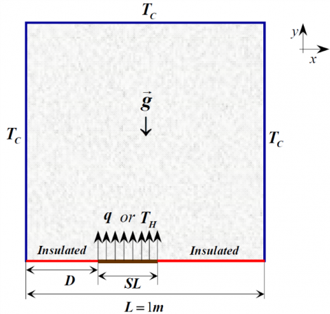
As described above, it is a natural convection problem in a square cavity filled with a Newtonian fluid (air), placed on a heat source of variable length SL and position D with respect to the left vertical side wall. Two thermal heating types for the source are supposed. The first: q-imposed, where a heat flux is delivered by the source inside the cavity with a uniform density q. The second: T-imposed, where the source is at hot uniform temperature TH. All the remaining walls are kept at low temperature TC. For source length lower than 1.0, the remaining parts of the bottom wall are insulated (Figure 1).
Figure 1. Geometry and details
The regime is assumed to be laminar with constant physical properties except for density, assumed variable with temperature (ρ=ρref(1-β(T-Tref)). Prandtl is taken equal 0.71. The problem of two-dimensional and Cartesian. After having adopted the Boussinesq hypothesis, the problem equations are as follows:
$\frac{\partial {{u}_{1}}}{\partial x}+\frac{\partial {{u}_{2}}}{\partial y}\text{=0}$ (1)
${{u}_{1}}\frac{\partial {{u}_{1}}}{\partial x}+{{u}_{2}}\frac{\partial {{u}_{1}}}{\partial y}\text{=}-\frac{1}{{{\rho }_{ref}}}\frac{\partial p}{\partial x}+\frac{\mu }{{{\rho }_{ref}}}\left( \frac{{{\partial }^{2}}{{u}_{1}}}{\partial {{x}^{2}}}+\frac{{{\partial }^{2}}{{u}_{1}}}{\partial {{y}^{2}}} \right)$ (2)
$\begin{align} & {{u}_{1}}\frac{\partial {{u}_{2}}}{\partial x}+{{u}_{2}}\frac{\partial {{u}_{2}}}{\partial y}\text{=}-\frac{1}{{{\rho }_{ref}}}\frac{\partial p}{\partial y} \\ & +\frac{\mu }{{{\rho }_{ref}}}\left( \frac{{{\partial }^{2}}{{u}_{2}}}{\partial {{x}^{2}}}+\frac{{{\partial }^{2}}{{u}_{2}}}{\partial {{y}^{2}}} \right)+g\beta \left( T-{{T}_{ref}} \right) \\ \end{align}$ (3)
${{u}_{1}}\frac{\partial T}{\partial x}+{{u}_{2}}\frac{\partial T}{\partial y}\text{=}\frac{k}{{{c}_{p}}.{{\rho }_{ref}}}\left( \frac{{{\partial }^{2}}T}{\partial {{x}^{2}}}+\frac{{{\partial }^{2}}T}{\partial {{y}^{2}}} \right)$ (4)
where, u1, u2: Velocity components following x and y respectively; p: Pressure; T: Temperature; g, β, cp and k: Gravity, thermal expansion coefficient, specific heat capacity and thermal conductivity respectively; ref: indicates values at reference temperature supposed here TC.
To quantify and qualify the effects density temperature-dependence, the source length and position, the Rayleigh number (Ra) was determined. It is calculated by the following expression (according to the heating condition):
$\begin{align} & {{\left. Ra \right|}_{q}}={\rho _{ref}^{2}\,{{c}_{p}}g\beta {{L}^{3}}\Delta T}/{(k.\mu )}\;\,\,;\,\,\,\,\,\,\,\,\,\,\,\,\,\,\,\,\,(\Delta T={qL}/{k}\;) \\ & \left. Ra \right|{{\,}_{T}}={\rho _{ref}^{2}\,{{c}_{p}}g\beta {{L}^{3}}({{T}_{H}}-{{T}_{C}})}/{(k.\mu )}\; \\ \end{align}$ (5)
For the source length and position, they are mentioned directly with the dimensional values since we took a cavity side of 1.0 meter of length.
Boundary conditions:
With the previous details, the problem corresponding boundary conditions are as follows:
$\begin{align} & \left( x=0\,\,or\,\,L,y \right)\to {{u}_{1}}={{u}_{2}}=0\,\,;\,\,T={{T}_{C}} \\ & \left( x,y=L \right)\to {{u}_{1}}={{u}_{2}}=0\,\,;\,\,T={{T}_{C}} \\ & \left( x=0\to D\,and\,(D+SL)\to L,y=0 \right)\to {{u}_{1}} \\ & ={{u}_{2}}=0\,;\,\,{\partial T}/{\partial y}\;=0 \\ & \left( x=D\to D+SL\,,y=0 \right)\to {{u}_{1}}={{u}_{2}} \\ & =0\,\,;\,\,{\partial T}/{\partial y}\;={q}/{r}\;\,\,\,or\,\,{{T}_{H}} \\ \end{align}$ (6)
It is important to note that originally, the problem is 3D, whit square source placed in a cubic cavity on the center of the lower facet. For a centered source, results along x and z are the same, and the problem becomes 2D. For a source outside the center but with displacement along x direction, only changes along x and y are important to analyze.
2.1 Heat transfer coefficient
The variation of temperature in the cavity and on the source leads to a variable convective heat exchange rate, for this, the calculation of the local Nusselt number is necessary. For the present problem, it has the expression:
${{\left. Nu \right|}_{q}}={q.L}/{({{T}_{Source}}-{{T}_{C}})}\;\,\,\,\,;\,\,\,\,\,{{\left. Nu \right|}_{T}}={{\left. {\partial \theta }/{\partial y}\; \right|}_{y=0}}$ (7)
With: $\boldsymbol{\theta}=\left(T-T_{C}\right) /\left(T_{S}-T_{C}\right)$
TSource, is the source temperature gotten from simulation.
This local Nusselt (mentioned Nu in the results) will be used to calculate the average Nusselt number more representative for the whole exchanged thermal flux. This latter is calculated using the following expression:
$\overline{Nu}=\frac{1}{SL}\int\limits_{D}^{D+SL}{Nu.\,}dx$ (8)
For all the dimensionless numbers, the cavity side length (L) was taken as characteristic length.
Conservation mass, momentum and energy equations, are solved numerically using a finite volume code. A second-order central differencing scheme is used for the diffusive terms, while a second-order up-wind scheme is used for the convective terms. SIMPLE Algorithm [12] is employed to treat the coupled’ pressure-velocity set of equations. Convergence residual values, are chosen 10-6 for mass and momentum parameters, and 10-9 for energy one. PISO Algorithm with two Skewness and neighbor corrections was used for some simulations for calculation stability.
3.1 Optimal mesh and validation
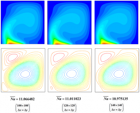
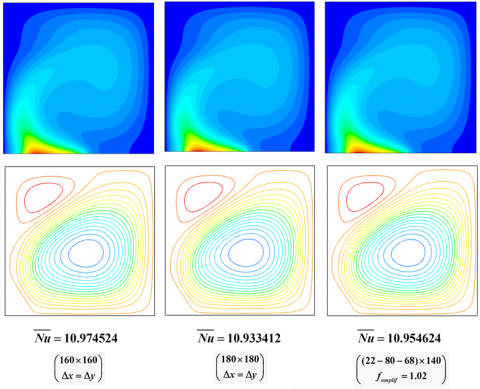
Optimal mesh (Figure 2) selection was done after a preliminary study of dependence of the results to the mesh, which was carried out, by using an equidistant mesh in both directions progressively refined, then make comparison with a non-uniform mesh, very refined on the source (x direction) and close to the walls by exploiting the physics of the problem (Figure 3), allowed us to arrive at the choice of our optimal mesh, that ensures excellent results for reduced time of calculation. This mesh is characterized by: ∆y=1/140, for the source: ∆xS=1/200 and for the insulated parts ∆xIn≈1/150.
Figure 2. Mesh refinement effect on thermal, velocity fields and average Nusselt number and comparison with the optimal chosen mesh. Ra=10+6; Pr=0.7; SL=0.4; D=0.15
Figure 3. Representative picture of the optimal mesh for SL=0.4 and D=0.15
So, for a centered source with length equal 0.1m (or 0.1 shortly), the mesh will be ((68-20-68)x×140y). This mesh offers more refinement on the source that generates the flow inside the cavity without messing a good mesh for the remaining zones. We notice that an amplification factor equal to 1.02 from both sides of each segment was used to well catch flow and temperature gradients, reduce cells number and get a smooth transition between them. For our simulations, the meshes used for a source in the middle of the lower wall are:
SL=0.1: 68-20-68×140; SL=0.2: 60-40-60×140; SL=0.4: 45-80-45×140;
SL=0.6: 30-120-30×140; SL=0.8: 15-160-15×140; SL=1.0: 180×140.
A rearrangement between the isolated parts is done when the source is out of the center.
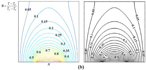
After choosing the optimal mesh, many validations were made, to be confident with the new results provided here. We present here only three validations of large significations, to avoid producing several ones, in order to save the work size. For all validations, the cavity top wall is insulated. The first validation (Figure 4), is done with the work of Saha et al. [11], for the temperature field for three values of Gr (Grashof number) and two values of SL. We note that for this case, the source is placed in the center of the bottom wall and is under imposed temperature (TH). The second validation (Figure 5) made for the values: Pr=100, Gr=10+6 and SL=0.4. In this validation, we tested our calculations with those of Raisi [9]. The source is under a heat flux density (q). This validation focuses on the positional effect of the source, where three positions were taken. Almost identical results were found for both validations. It should be noted that we did not present the streamlines profiles because of the very limited details in the two references. The third presented validation is for $\overline{N u}$, for two values of SL and different values of Gr. The comparison is made with values calculated by Sharif and Mohamed [10] and Saha et al. [11] for SL=0.2, and only with reference [10] for SL=0.8 (Table 1). Very good results have been obtained.
Table 1. Some validations for the mean Nusselt number
|
|
Ra=10+3 |
Ra=10+4 |
Ra=10+5 |
Ra=10+6 |
|
S=0.2 (D=0.4); Pr=0.71 |
||||
|
$\overline{N u}$ |
5.93017 5.92661[10] 5.939[11] |
5.96653 5.94635[10] 5.954[11] |
7.14559 7.12406[10] 7.114[11] |
11.41132 11.3415[10] 11.226[11] |
|
S=0.8 (D=0.1); Pr=0.71 |
||||
|
$\overline{N u}$ |
3.64596 3.55618[10] |
3.76584 3.69192[10] |
5.92884 5.86442[10] |
9.37324 9.28797[10] |
Figure 4. Validation for temperature field. T-imposed; Source at the center; Pr=0.71; (a): SL=0.4/Gr=10+6; (b): SL=0.4/Gr=10+3; (c): SL=0.2/Gr=10+4. (Left: Our results; Right: Results of Saha et al. [11])
Figure 5. Validations for temperature field. q-imposed; Gr=10+6; Pr=100; SL=0.4. (a): D=0.0; (b): D=0.1; (c): D=0.2. (Left: Our results; Right: Results of Raisi [9]).
For a better exploitation of the results obtained and to illustrate the effects of the many intervening parameters, this part of the work is divided into three parts, in which we first present and discuss the effects of Ra and SL on the temperature (isotherms) and velocity fields (current lines) for the classic case with source at the center of the lower wall. The effect of D while varying the two previous parameters is analyzed in the second part. The results for Nu (Local Nusselt number) and $\overline{N u}$ (Average Nusselt number) are presented after those for isotherms and streamlines. It is very useful to avoid any misunderstanding, in addition to not weigh down the paper, to mention that we will present the case of source under heat flux heating type (q-imposed) at first with maximum details. The results for the case of a temperature imposed at the source (T-imposed) will be summarized for the temperature and velocity fields, considering the similarity with those of the first type of heating. In the third part, we presented results on the effect of increasing the Prandtl number (Pr) on the intensity of the local and averaged heat exchange rate, where a detailed discussion was given.
4.1 Effects of Rayleigh number (Ra) and source length (SL) for a source at the center
In this part, the heat source is placed exactly in the center of the bottom wall. The effects of the Rayleigh number (Ra) and the length of the source (SL) will be analyzed.
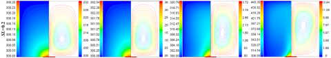
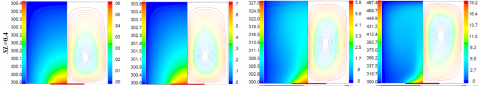
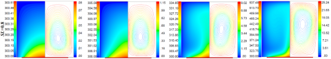
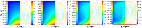
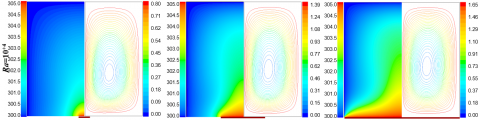
Figure 6 shows the effects of the change of Ra (convection intensity) and SL (source length) on the isothermal profiles and current lines. Four values of Ra (10+3, 10+4, 10+5 and 10+6) and six SL values (0.1, 0.2, 0.4, 0.6, 0.8 and 1.0) were taken. For this figure, the source is under uniform heat flux (q-imposed). By analyzing the thermal field, we can see the location of the red zone (very hot) on and very close to the source as expected, a transition to the dark blue (very cold zone) which represents the TC temperature, passing through the yellow, green and light blue which translate the temperatures between the maximum temperature at the source and the minimum temperature at the cold walls. The good analysis of the sub-figures shows that the maximum value lies exactly in the center of the source by symmetry.
For the low values of Ra (10+3 and near), we can see that the isotherms have a convex shape reflecting the smooth propagation of heat when the mode is almost conductive. It should also be noted that heating is becoming more important as SL length increases due to the larger area from which heat enters. For this, we see thicker light blue areas. By slightly increasing Ra (10+4 and near), we can see small perturbations in the field of isotherms from SL=0.4 and larger. This is due to the natural convection generation with a sufficient degree because of the high temperatures which decrease the density of the fluid by a sufficient level. It is obvious that this phenomenon becomes stronger when SL increases. By further increasing Ra (increase of β or Tsource), disturbances are observed for all SL values. A net of hot fluid joins the upper part and reaches the upper wall and eventually deflects symmetrically with respect to the vertical plane of symmetry located in the source’ center. Hot currents will reach the two side walls from where a better distribution of the temperature.
The velocity field presented by the streamlines is directly affected by the increase of Ra, because of the coupling of the problem. Increasing intensities are reached when Ra increases (see legends). Since the flow is generated due to the decrease in density of the fluid with the increase in temperature and the latter is higher near the source and increases with SL. Increasing intensities with SL are also recorded. The association of the effect of Ra with that of SL thus offers a maximum of intensity of the natural convection flow. In addition, a movement of the circulation zones upwards when Ra and/or SL increase is observed following the strong disturbance which causes the hot fluid stream to be launched in the center of the source upwards.
Figure 7 shows the temperature velocity fields for the T-imposed heating type, where the source is under the constant temperature TH. Only six cases were presented, where two values were taken for Ra, 10+4 representing a low temperature dependence of the density and 10+6 for the opposite case, and three SL values ranging from the smallest (0.1) to the longest one (1.0) through an average length (0.4).
The sub-figures analysis shows the reproduction of the same observations of the previous type of heating, as expected physically. We notice the faster beginning of disturbances in the cavity for this case compared to the previous one.
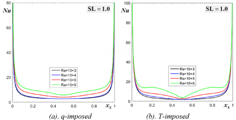
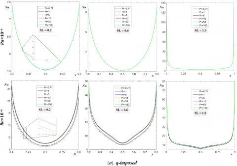
The local Nusselt number (Nu) evolution along the source for the two types of heating is presented in Figure 8. Three cases were presented for each type, where we took three source’ length, SL = 0.2, 0.6 and 1.0 and four values of Ra (10+3, 10+4, 10+5 and 10+6), for the same reason considered for Figure 7. As expected, the increase in flow disturbance generates a growth in the intensity of heat exchange. This is clearly observed on the sub-figures. But we note that the T-imposed heating type (TH) offers more convective heat exchange rate following the strong disturbance as mentioned above. The curves analysis for both heating types shows that a maximum Nu value is recorded at the ends of the source and a minimum exactly at the center of the latter. This is explained by the fact that the value of Nu increases with the decrease of the temperature of the fluid near the source which allows the introduction of more heat flow from it, and since the maximum temperature is exactly in the center of the source, the minimum of Nu will be there and conversely at the source ends.
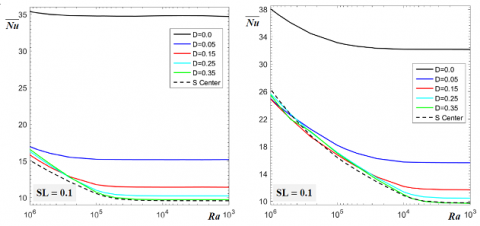
In Figure 9, mean Nusselt evolution ($\overline{N u}$) is presented as a function of the Rayleigh number (Ra) for the six SL values considered and for both types of heating. It is noted that in order to plot the curves, twenty-five Ra values were used in simulation for each case (10+3, 1.25×10+3, 2.5×10+3, 5×10+3, 6.25×10+3, 7.5×10+3, 8.75×10+3, 10+4,…, 10+6). This high number provides good accuracy of the results. As expected, it is clear that heat exchange decreases with the decrease of Ra. Moreover, and from the curves, one can see that for all the cases, there is a passage point from a purely horizontal curve (slope null) to an inclined curve (negative slope). The purely horizontal part represents the non-sensitivity of the density of the fluid to the increase of Ra. In other words, it is only from a certain value of Ra that the difference in the disturbances of the flow changes by a clear degree. In summary, the point between the two parts, horizontal and inclined, changes clearly with the source length SL for q-imposed case, where the Ra corresponding value becomes smaller when SL increases following the increase of the temperature of the source and vice versa. For the T-imposed case, this point does not depend on SL, since the source temperature is the same for all lengths (TH) at same Ra, hence the equitable change in density whatever SL is. It is the value of Ra itself (increase of β or TH) which will cause the change in the curve shape.
The most important result in this first part is the better heat exchange rate for SL=0.1 compared to all other cases. The second best exchange is obtained for SL=1.0 followed by 0.2, 0.4, 0.6 and finally 0.8. A very strong fall between the case at SL=0.1 and SL=0.2 is recorded. In our opinion, this is an observation that deserves a detailed study to properly analyze the cause of this jump. For the physical explanation, we start with the case SL=1.0. As previously discussed, the heat exchange increases with Ra following the growth of the dependence of the density at β and/or TSource. The second parameter influencing the heat exchange rate is the condition of cold walls under temperature TC which is the lowest temperature in all the geometry. For this, the fact of taking SL=1.0, leads to the direct contact between the source which represents the entire lower wall with the side walls both under TC. Therefore, it is obvious to have a better exchange compared to the case where the source is far from the side walls (i.e SL<1.0), so that the path of the hot fluid is very short for SL=1.0 compared to the others, which leads to the rapid extraction of the heat flux released by the source in the fluid medium. When SL begins to be less than 1.0, friction between the fluid and the wall (increases with SL) which is larger than that between the upward and the downward cold fluid opposes the natural convection flow, which results in lower values of $\overline{N u}$ for SL=0.8 than SL=0.6 and so on until SL=0.1. The case SL=1.0 does not escape this rule, but we must not forget that the temperature of the source increases with SL and the maximum of TSourceis recorded for this case (an effect opposing the braking thus results).
But, the case of SL=0.1 offers a very strong $\overline{N u}$, bigger even than that of SL=1.0 which has the advantage of the contact of the source with the cold side walls. It is believed that the short length of the source provides a large spacing between the source and the two walls, which neglects the friction effect experienced by the other SLs to the maximum. In addition, the small size of the source is that it is mostly surrounded by the cold fluid, which causes the heat released by the source to disperse in the fluid easily. From the results, there exists a length SL between 0.1 and 0.2 for the case q-imposed at the source where $\overline{N u}$ equalizes that for SL=1.0. The explanation given is valid for the first type of heating (q-imposed) and is valid only for low or medium Ra for the second type of heating (T-imposed). For the strong Ra, we observe that $\overline{N u}$ decreases with SL including SL=1.0. The explanation that can be given is the fact of supposing TH fixed at the source, the length does not influence the temperature of the source (unlike the case q-imposed), and it is the distance of the source at the side walls that motivates the improvement or degradation of $\overline{N u}$. For people who are most interested in cooling itself, it is advisable to ensure that you have a minimum source length (SL<0.2) at high Ra if possible, for both types of heating. For a low or medium Ra, care must be taken to further reduce the length of the source.
Figure 6. Effect of Ra and source length SL on temperature (Left half) and stream-functions (Right half). Source at the center. q-Imposed. Pr=0.71
Figure 7. Effect of Ra and source length SL on temperature (Left half) and stream-functions (Right half). Source at the center. T-Imposed. Pr=0.71
Figure 8. Local Nusselt (Nu) variation along the source for different Ra and SL. Source at the center. Pr=0.71
Figure 9. Mean Nusselt ($\overline{N u}$) variation according to Rayleigh number (Ra) for different source’ length (SL). Source at the center. Pr=0.71
4.2 Effect of source position (distance D with respect to the left side wall)
In this part, we have varied the position of the source, starting from the left side corresponding to D=0.0 towards the center, with value of D changeable with the length SL. The first movement step is taken 0.05, then 0.1 until reaching the source position in the center.
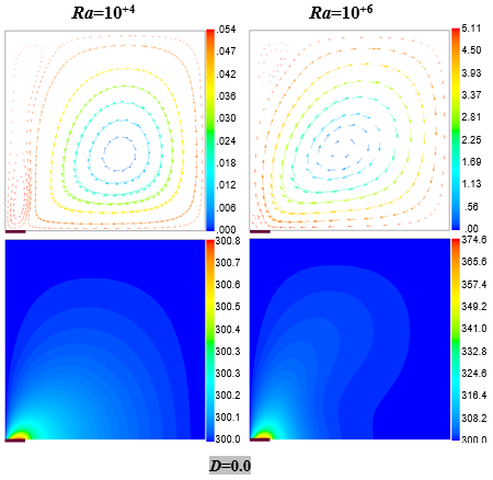
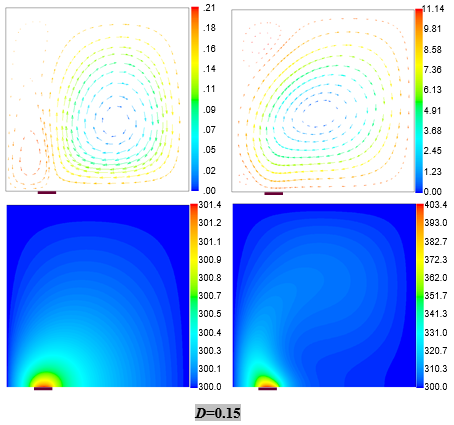
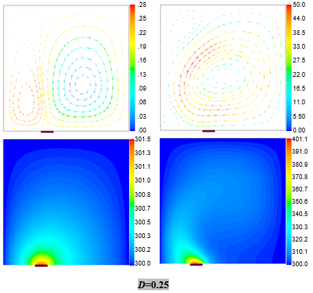
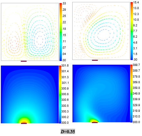
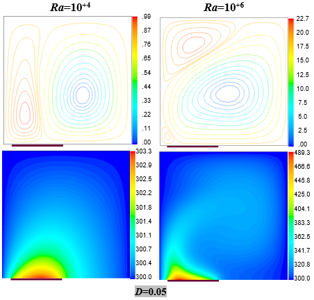
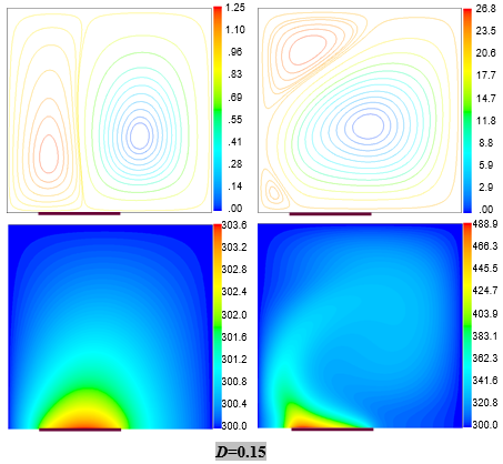
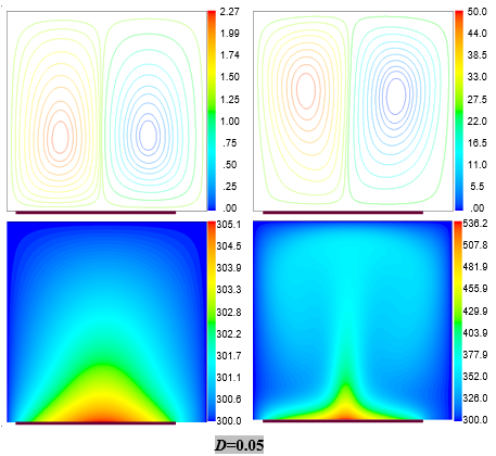
In Figure 10, the results of the thermal (Isotherms) and dynamic (current lines) fields were presented for different positions of the source. We took three lengths SL=0.1, 0.4 and 0.8 and two values of Rayleigh, Ra=10+4 and 10+6, which are sufficiently numerous while ensuring a gain of space. As followed in the paper, the results are for the q-imposed case only. Those of the T-imposed case are not presented because of the resemblance as shown in Figures 6-7. The first logical remark is the disappearance of symmetry when the source is no longer in the middle of the lower wall, especially when D is close to 0.0. Starting with the case of SL=0.1, where it is observed that for low values of Ra, a long circulation zone above the source, characterized by a small width with fluid currents rotating counterclockwise. The majority of fluid rotates in the opposite direction (hourly), by continuity in the cavity. The arrows used for the case SL=0.1 help to better see the circulations for this case and imagine those of the other two presented (0.4 and 0.8). The circulation zone that has been lengthened along the vertical becomes localized in the lower left and upper corners when Ra increases, under the effect of the strong circulation of the rising hot fluid which reaches the left wall once it finds a little freedom of movement not possible at the two corners. It is worth to note that we intentionally avoided presenting the case of source at the center for SL=0.4 and SL=0.8 (Figure 10), in order to provide suitable presentation and save space. Figure 6 can be consulted for these two cases.
When the distance D increases (SL=0.1), the fluid counterclockwise rotating zone widens gradually but remains smooth for the weak Ra. For the strong Ra, the two small circulation zones widen with greater degree for the upper one once the path of the fluid deviates by spacing between the source and the left wall at the bottom which modifies the pace of the flow. For average source lengths (close to SL=0.4), the above phenomena remain globally valid while noting a much larger zone in the upper corner for the strong Ra, following the higher temperatures reached on the source under the effect of the length. For SLs close to 1.0 (SL=0.8 and near), the two previously observed zones for the strong Ra unite in one zone because almost the entire lower zone near the source is the seat of the rising warm fluid. The long length SL reduces the effect of its approximation regarding the left side wall (D effect weakened).
(a). SL=0.1
(b). SL=0.4
(c). SL=0.8
Figure 10. Source position (D) effect on stream-functions (upper square) and temperature (lower square) for Ra=10+4 and 10+6 and three source lengths SL=0.1, 0.4 and 0.8. q-Imposed. Pr=0.71
For the temperature field and given the coupling of the problem, a slightly regular temperature field is recorded for the weak Ra with deviation to the right of the hot fluid, direction of the majority of the flow. For the strong Ra, a clear disturbance of the temperature field, where two situations are distinguished: for the distances D close to 0.0, the hot fluid is deviated to the right with disturbed pace compared to the weak Ra; for larger distances, the hot fluid undergoes a deviation to the left then to the right under the effect of the widening of the two circulation zones recorded in the low and high corners as discussed for the velocity field. An almost symmetrical pace is observed for SL=0.8 (and close) as expected even at high Ra.
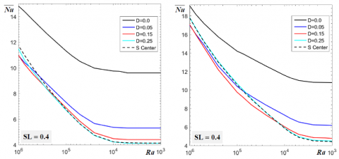
The observed changes in the velocity and temperature fields result, of course, in changes in the mean convective exchange coefficient presented in Figure 11. It is noted that each result curve is plotted from 13 simulation values for Ra (10+3, 2.5×10+3, 5.0×10+3, 7.5×10+3, 10+4, …, 10+6). In addition, the presentation of the variation of the local Nusselt (Nu) was avoided by intention. The first reason is that it is clear that it is no longer symmetrical with respect to the center of the source and its evolution is the opposite of that of the source temperature as discussed in Figure 8. The analysis of temperature sub-figures offers enough information for the one interested. The second reason is the large number of cases to be presented, and finally, it is the average exchange rate ($\overline{N u}$) that really interests us because it reflects the average global exchange rate.
Figure 11. Mean Nusselt ($\overline{N u}$) variation according to Rayleigh number (Ra) for different source’ length (SL) and position (D). Pr=0.71
Figure 12. Local Nusselt (Nu) variation along the source for different Prandtl number (Pr) and source’ length (SL). Source at the center
The curves of the latter shown in Figure 11, show that the maximum exchange is for D=0.0 for all simulated SLs and for both types of heating. Not only this, but its value is significantly higher, which offers a result of great practical importance. It is thought that it is because of the location of the source in contact with the left side wall under TC that the exchange has improved. Moving away from this wall, the rate will gradually decrease when D increases, where it is observed that the classical case with source in the center of the lower wall leads to the lowest heat exchange rate. The improvement of $\overline{N u}$ with the displacement towards the cold side wall is valid mainly. Some cases with strong Ra are exceptions without expected way. It is thought that this is because of the perturbations observed in the fields of velocity and temperature. But, the case at D=0.0 remains the best regardless of Ra and/or SL.
It is important to mention that for the q-imposed heating type with D=0.0 and SL=0.1, there is almost no sensitivity to the increase of Ra. In our opinion, it is the combination of contact with the wall that dissipates the heat flow entering through the cold side wall, in addition to the very small size of the source that maximizes the surrounding cold fluid. The T-imposed case has a slight sensitivity for the same detailed causes for the case of a source at the center.
4.3 Effect of Prandtl number (Pr)
For this last part, we will analyze the effect of the Prandtl number (Pr) on the local heat exchange rate (Nu) along the source, then the average one ($\overline{N u}$). To do this, the results of the local Nusselt (Nu) were obtained by taking six values for Pr (0.71; 1.0; 5.0; 10.0; 50.0 and 100.0), two values of Ra (10+4 and 10+6) which represent small and large intensities of convection and three values of the source length SL (0.2; 0.6 and 1.0). We note that we took Pr=100.0 as the maximum value because of the non-sensitivity of the results (uninfluenced thermal and dynamic fields) for higher values. Turan et al. [13-15] offer sufficiently rich and clear details on this subject.
The analysis of the local Nusselt (Nu) curves in Figure 12 shows that the effect of Pr is negligible for low values of Ra (10+4 and near). This seems logical, since its effect is opposite to that of Ra, which is still small and therefore little sensitivity of the flow to the change of Pr. By increasing Ra, the natural convection flow intensifies as detailed in section 4.2 and any opposition will be clear, especially if its cause amplifies as one can see on the sub-figures for Ra=10+6. For this, in this case (Ra=10+6) one can see the separation of Nu’ lines representing the different values of Pr from each other, with increasing magnitude when Pr increases. It is obvious that this observation remains valid for other values of Ra close to 10+6. The explanation of this improvement is the widening of the zones disturbed by the flow generated by natural convection, under the increasing effect of the viscosity and/or the decreasing one of the thermal diffusivities (Pr=ν/α). This implies that there will be larger heat diffusion in the cavity when Pr increases by transmission of the natural convection effect to more distant areas. Therefore, a better heat transfer rate results due to the greater heat diffusion, which causes a decrease in temperatures near the source and hence more introduced heat flux from it. This explanation is valid for both thermal conditions imposed on the source (Figure13). Two important results can be drawn from Nu's evolution (Figure12). The first is the limitation of the effect of Pr after a certain degree (Pr≈50), for the reason we have just discussed. The second is its stronger effect near the center of the source compared to its extremities. This result seems very obvious because the convection flow that is generated close to the source has its highest intensities near the source, where are recorded the largest values of the temperature, in addition that the areas near the ends of the source are at temperatures close to TC, hence, the low influence of Pr. This second result is loud and clear for a source under the q-imposed condition. For the second case (T-imposed), Pr effect is more pronounced on both sides of the center of the source than on the latter. Moreover, for large SL (≈1.0), one can see the crossing of Nu lines over a central distance from the source, then a high increase when Pr increases. This is explained by the change in the form of the isotherms very close to the source (it is recalled that for this case of heating, the whole source is under the same temperature, it is his entourage which undergoes the modification) compared to the case q-Imposed where the form remains similar when Pr changes (reconsider Figure 13).
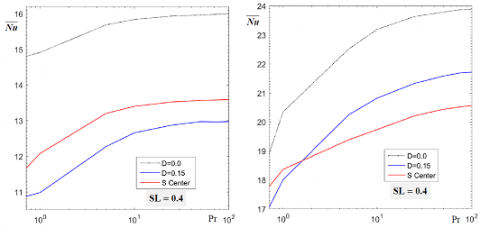
In Figure 14, the mean Nusselt ($\overline{N u}$) evolution is presented for different SL values (0.1, 0.4 and 0.8) as a function of Pr (0.71; 1.0; 5.0; 10.0; 25.0; 50.0; 75.0 and 100.0) and this for a single value of Ra (10+6), for the reason previously discussed (negligible effect of Pr for low Ra). As expected, a gradual improvement is obtained when Pr increases. One can observe a steep slope between Pr=0.71 and Pr=5.0, followed by another low and then a trend towards a horizontal evolution when Pr approaches and exceeds 50.0. From the figure, one can see that the increase influence of Pr is a little stronger for the T-imposed case than that of q-imposed. The explanation given for the local Nusselt remains valid here. In addition, the effect of Pr is present for all lengths and position of the source (different SL and D). It should be noted that the case with SL=0.1 and D=0.0 for a q-imposed heating, showed no sensitivity towards the increase of Pr. This in our opinion is explained by the small temperature values reached near the source because of the strong absorption of heat from the vertical wall in addition to the very short length of the source (reconsider Figure10). The second type of heating for the same characteristics (SL and D) showed a clear effect of Pr, because the source is under the same temperature TH even close to the vertical wall under TC.
Figure 13. Prandtl number (Pr) effect on temperature field. SL=0.6; Ra=10+6. Source at the center.
$\theta_{q}=\frac{\left(T-T_{C}\right)}{(q \cdot L / \lambda)} ; \theta_{T}=\frac{\left(T_{H}-T\right)}{\left(T_{H}-T_{C}\right)}$
Figure 14. Mean Nusselt ($\overline{N u}$) variation according to Prandtl number (Pr) for different source' length (SL) and position (D). Ra=10+6
The results obtained from the numerical simulation of the problem allowed us to conclude that:
- Effect of Pr number:
Finally, to better cool a heat source by means of a cold-walled square cavity, by exploiting the dependence of the fluid density of the temperature, it is recommended to choose the side size more than five times that of the source. Place the source in contact with one of the vertical sides and preferably use fluids with Pr>50.0 to maximize the heat exchange rate. But everything depends on the needs, the objectives, the availability of means and the cost of integration.
|
Cp |
Specific heat (J .Kg-1.°C -1) |
|
D |
Distance between the source left extremity and the vertical left side (m) |
|
g |
gravitational acceleration, m.s-2 |
|
k |
Thermal conductivity (J/s. m.°C) |
|
L |
Cavity side length (m) |
|
Nu |
Local Nusselt number |
|
$\overline{N u}$ |
Mean Nusselt number |
|
p |
Pressure (Kg/m.s-2) |
|
q |
Heat flux density (J/s.m²) |
|
Ra |
Rayleigh number |
|
SL |
Source length (m) |
|
T |
Temperature (°C) |
|
u1 |
x-velocity component (m/s) |
|
u2 |
y-velocity component (m/s) |
|
x |
x-coordinate |
|
y |
y-coordinate |
|
Greek symbols |
|
|
ρ |
Fluid density (Kg .m-3) |
|
θ |
Dimensionless temperature |
|
β |
Thermal expansion coefficient (1/°C) |
|
µ |
Viscosity (Pa.s) |
|
Subscripts |
|
|
C |
Cold |
|
H |
Hot |
|
ref |
Reference |
[1] Öztop, H.F., Estellé, P., Yan, W.M., Al-Salem, K., Orfi, J., Mahian, O. (2015). A brief review of natural convection in enclosures under localized heating with and without nanofluids. International Communications in Heat and Mass Transfer, 60: 37-44. https://doi.org/10.1016/j.icheatmasstransfer.2014.11.001
[2] Baïri, A., Zarco-Pernia, E., De María, J.M.G. (2014). A review on natural convection in enclosures for engineering applications. The particular case of the parallelogrammic diode cavity. Applied Thermal Engineering, 63(1): 304-322. https://doi.org/10.1016/j.applthermal eng.2013.10.065
[3] Rahal, S., Begar, A., Hamada, A. (2017). Numerical study of natural convection in a cavity filled with air and heated locally from below. International Journal of Applied Mathematics Electronics and Computers, 5(1): 20-24.
[4] Banerjee, S., Mukhopadhyay, A., Sen, S., Ganguly, R. (2008). Natural convection in a bi-heater configuration of passive electronic cooling. International Journal of Thermal Sciences. 47: 1516-1527. https://doi.org/10.1016/j.ijther malsci.2007.12.004
[5] Seddiki, M.N., Habiba, F., Chowdhury, R. (2017). Effect of buoyancy force on the flow field in a square cavity with heated from below. International Journal of Discrete Mathematics, 2(2): 43-47. https://doi.org/10.11648/j.dmath.20170202.13
[6] Aydin, O., Yang, W.J. (2000). Natural convection in enclosures with localized heating from below and symmetrical cooling from sides. International Journal of Numerical Methods in Heat and Fluid Flow, 10(5): 519-529.
[7] Calcagni, B., Marsili, F., Paroncini, M. (2005). Natural convective heat transfer in square enclosures heated from below. Applied Thermal Engineering, 25: 2522-2531. https://doi.org/10.1016/j.applthermaleng.2004.11.032
[8] Sarris, I., Lekakis, I., Vlachos, N. (2004). Natural convection in rectangular tanks heated locally from below. International Journal of Heat and Mass Transfer, 47: 3549-3563. https://doi.org/10.1016/j.ijheatmasstransfer.2003.12.022
[9] Raisi, A. (2016). Natural convection of non-Newtonian fluids in a square cavity with a localized heat source. Journal of Mechanical Engineering Science, 62(10): 553-564. https://doi.org/10.5545/sv-jme.2015.3218
[10] Sharif, M.A.R., Mohammad, T.R. (2005). Natural convection in cavities with constant flux heating at the bottom wall and isothermal cooling from the sidewalls. International Journal of Thermal Sciences, 44: 865-878. https://doi.org/10.1016/j.ijthermalsci.2005.02.006
[11] Saha, G., Saha, S., Islam, M., Akhanda, M. (2007). Natural convection in enclosure with discrete isothermal heating from below. Journal of Naval Architecture and Marine Engineering, 4: 1-13. https://doi.org/10.3329/jname.v4i1. 912
[12] Patankar, S.V. (1982). Numerical Heat Transfer and Fluid Flow. Hemisphere, Washington, DC. https://doi.org/10.1002/cite.330530323
[13] Turan, O., Poole, R.J., Chakraborty, N. (2011). Influences of boundary conditions on laminar natural convection in rectangular enclosures with differentially heated side walls. International Journal of Heat and Fluid Flow, 33(1): 131-146. https://doi.org/1080/01457632.2014.852870
[14] Turan, O., Sachdeva, A., Poole, R.J., Chakraborty, N. (2001). Laminar natural convection of power-law fluids in a square enclosure with differentially heated side walls subjected to constant wall heat flux. Numerical Heat Transfer, Part A, 134(12): 381-409. https://doi.org/10.1080/10407782.2011.594417
[15] Horimek, A., Noureddine, B., Benkhchiba, A.E., Ait-Messaoudene, N. (2017). Laminar natural convection of power-law fluid in a differentially heated inclined square cavity. Annales de Chimie -Science des Matériaux, 41(3-4): 261-281. https://doi.org/10.3166/ACSM.41.261-281