Vittorio Ferraro* | Valerio Marinelli | Jessica Settino | Francesco Nicoletti
© 2020 IIETA. This article is published by IIETA and is licensed under the CC BY 4.0 license (http://creativecommons.org/licenses/by/4.0/).
OPEN ACCESS
In this study, a simplified calculation method to evaluate the thermodynamic performance of two solar tower power plants of 50 MW is proposed. The systems consist in an open air Brayton cycle and a Brayton-Rankine combined cycle. The electricity produced, the average annual efficiency of the heliostats field-receiver system, the efficiency of the thermodynamic cycle and of the entire plant have been determined for both systems. The performances of the two plants have been compared to conventional plants using molten salts. The analysis shows that both systems have better performances than conventional solar tower plants using molten salts. The specific annual electrical energy per square meter of heliostat is higher than that obtained for the plant using molten salts, by 11.5% and 38.7% for the Brayton and the Brayton-Rankine combined cycle respectively. Moreover, an economic analysis has been performed. The results show that a reduction of the Levelized cost of Electricity (LCOE) can be achieved compared to the traditional molten salt plants, with savings of 15% and 13.6% for the Brayton and combined cycle respectively.
combined cycle, open air Brayton cycle, solar tower plants, thermodynamic performance, economic analysis, levelized cost of electricity
This work is an update of the previous paper on solar tower power plants [1]. Solar energy represents an attractive source for electricity generation [2] and the interest in the CSP technology is increasing worldwide [3, 4]. An overview of different solar thermal power plants is provided by Siva Reddy et al. [5]. Xu et al. [6] analysed the main challenges of concentrating solar power plants in desert areas. Boretti et al. [7] focused their analysis on concentrating solar tower technologies. The authors provide an update on the current status, the actual costs and operation of solar tower systems.
The most common type of concentrating solar tower power plant is the one that uses molten salt as both heat transfer fluid and thermal storage medium. This plant is provided with a salt-water steam generator that feeds the power block operating with a water steam Rankine cycle [8, 9].
For some years there has been an increasing interest in the possible use of gases, including helium, neon, argon, carbon dioxide, nitrogen, air, as heat transfer fluids in solar receivers. Gases have lower densities than liquids and therefore they present higher pressure drops and higher pumping powers than those of molten salts. It is possible to overcome this disadvantage by increasing the gas operating pressure. At Plataforma Solar de Almeria (PSA), pressure drops and pumping power measurements for helium, nitrogen, carbon dioxide and air were carried out in an experimental setup consisting of two 50 m linear parabolic collectors connected in series or in parallel in a closed hydraulic circuit [10]. Owing to its excellent properties as heat transfer medium and because of its high density at high pressures, which reduces the pumping power, carbon dioxide under supercritical conditions (pressure greater than 73.86 bar) has proved to be the best gas to use in solar systems. Various studies [11-15] are reported concerning the performance of solar systems, both with parabolic collectors as well as with solar towers, employing carbon dioxide under supercritical conditions, confirming the advantages offered by this fluid. However, using carbon dioxide, there is the possibility of formation of carbonic acid, which is corrosive for carbon steel pipes. For this reason, a strict control of the moisture content is required [10]. Reyes-Belmonte et al. [16] compared the performance of a solar tower receiver coupled with different thermodynamic cycles: a subcritical steam Rankine cycle; a regenerative open air Brayton cycle; a combined cycle; a regenerative closed helium Brayton cycle and a recompression supercritical carbon dioxide Brayton cycle.
As an alternative to carbon dioxide, the use of atmospheric air as heat transfer fluid, evolving in a Brayton cycle or in a combined cycle, in plants with both parabolic trough collectors [17-19], and solar towers [20] has been proposed. The advantages of air with respect to all other heat transfer fluids are very clear: air is inexpensive, completely safe, and non-pollutant; moreover, no water is required, which is a very attractive prospective in arid climates.
The first experiments with air were carried out at PSA in 2003, by using the first prototype hybrid solar powered 230 kW gas turbine system. The solar receiver allowed to reach temperatures of 800℃ at the combustor air inlet [21]; then, other experiments were carried out in Newcastle, Australia, at the National Solar Energy Centre, where a 200 kW demonstration hybrid system with air Brayton cycle was constructed by the CSIRO agency [22-24]; moreover, the Abengoa Solar Company is performing experimental analysis on an air hybrid Brayton plant of 4.5MW [25, 26], provided with a 65 m tower and a receiver in which the air is heated up to 800℃ at Abengoa's Solúcar Platform near Seville.
The scientific literature on concentrating solar tower power plants operating with an open air Brayton cycle is still scarce, while there are few papers analysing the performance of air-water combined cycle solar tower systems [27-29].
A comparison of different concentrating solar technologies with integrated combined cycle has been performed by Rovira et al. [30]. The authors analysed two configurations. In one case, solar energy is used to evaporate part of the water in the Heat Recovery Steam Generator (HRSG). In the other case, the air at the compressor exit is pre-heated by the solar tower before entering the combustion chamber. An alternative configuration has been proposed by Amani et al. [31], the solar tower is used to heat up the exhaust gas from the gas turbine which are sent to the HRSG unit. Okoroigwe and Madhlopa [29] provided a review of integrated combined cycle coupled with a solar tower. The authors point out that, in spite of the progress in the Research and Development stage, there is no commercial solar tower with integrated combined cycle.
In this work, the thermodynamic performances of a solar tower power plant with an open air Brayton cycle (B plant) and a combined cycle have been analysed. Compared to other studies, the proposed systems are driven by solar energy only and no fossil fuels are used. A methodology to evaluate the performance of both systems in off-design conditions has been developed and an economic analysis has been carried out. The proposed solutions have been compared to a reference solar tower power plant with molten salts.
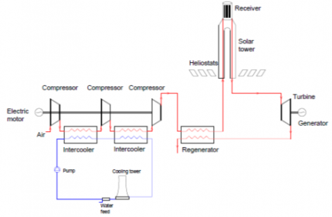
Figure 1 provides a schematic representation of a concentrating solar tower power plant with an open air Brayton cycle. The air drawn from the atmosphere is compressed by a three stage inter-refrigerated compressor, preheated in the regenerator and sent into the receiver placed on top of the solar tower, from which it exits at high temperature. Afterwards, it is sent to the gas turbine connected to the electric generator, and before being discharged to the atmosphere, the air passes through the regenerator. A cooling tower is used to refrigerate the water used in the cooling circuit.
Figure 1. Schematic representation of a solar tower power plant with an open air Brayton cycle
Figure 2 shows a concentrating solar tower plant with a combined cycle. It consists of a topping Brayton cycle, a heat recovery boiler and a bottoming Rankine cycle. The compressor sends the air directly into the receiver. The air at high temperatures drives the gas turbine. Afterwards, it is sent to a heat recovery steam generator, where superheated steam is produced and used to drive the steam turbine.
Figure 2. Schematic representation of a solar tower power plant with a Brayton-Rankine combined cycle
In both systems, a constant turbine inlet temperature (TIT) equal to 1000℃ is considered, while the flow rate varies depending on the direct normal radiation (DNI). When the flow rate reaches a threshold value, it is kept constant as the DNI decreases. In order to not degrade excessively the isentropic efficiency of the compressor, the minimum air flow rate should not be lower than 60% of its nominal design value. This determines a reduction of the turbine inlet temperature, up to a minimum value of 600℃, for which the plant can still produce electricity.
The operation of the components of the two systems was simulated by the THERMOFLEX code [32], starting from the design conditions, summarized in Table 1 and Table 5 and then evaluating their performances in off-design conditions, by varying the inlet temperature of the air and the opening of the Inlet Guide Vanes (IGV) of the compressor, so as to vary the air flow rate.
Based on the results obtained, some correlations have been developed for the key variables, such as the air temperature at the compressor exit in the combined cycle plant (or at the regenerator exit in the Brayton cycle) and the thermodynamic efficiency of the gas and steam turbines in the combined cycle (or of the gas turbine in the Brayton cycle).
At low solar irradiance, the plants are operated at constant flow rate, the correlations developed concerned the thermal power transferred to the fluid in the receiver, the air temperature at the inlet of the turbine, and the thermodynamic efficiency of the turbines.
All these correlations, along with a simulation model of the heliostat field and the tower receiver, were implemented in a Matlab calculation algorithm, called TERSOLTO (thermodynamic solar tower) in the B and CC versions, respectively valid for the Brayton cycle and the combined cycle.
Through TERSOLTO, starting from the values of direct solar irradiance, air temperature and humidity, the hourly values of the electrical power generated by the plants, the average hourly and annual values of the efficiency and the electricity produced in a year can be calculated.
In the following paragraphs the models and correlations used are described in detail.
2.1 Calculation model of the Brayton Cycle
Table 1 provides the main input data for the Brayton cycle: the rated electrical power, the atmospheric air temperature, the DNI design value, the inlet temperature to the gas turbine, the pressure ratio of the compressor and the turbine.
Once defined the type of system and characteristics of the various components, the THERMOFLEX code considers the receiver as a generic heat generator, and allows to calculate the nominal air flow rate. Hence, it is possible to obtain the desired net electrical power, the thermal power supplied from the receiver to the fluid, the gross and net electrical power supplied from the gas turbine, the net thermodynamic efficiency of the cycle and many other variables of interest.
By means of the THERMOFLEX code, after determining the above mentioned variables in design conditions, calculations in off-design conditions were performed, considering: three different values of the atmospheric air temperature of 0℃, 25℃ and 50℃; three opening values of the IGV, of 100%, 80% and 60%; and maintaining the turbine inlet temperature constant at 1000℃.
Table 1. Design data of Air Brayton Solar Tower Power Plant located in Almeria
|
Parameter |
Value |
|
Nominal net electrical Power |
50 MW |
|
Direct Normal Irradiance (DNI) |
850 W/m2 |
|
Zenith angle |
13.850° |
|
Azimuth angle |
-10.713° |
|
Total area of heliostats |
302,499 m2 |
|
Reflectivity of heliostats |
0.94 |
|
Absorptivity of receiver |
0.97 |
|
Optical efficiency of heliostats field |
0.567 |
|
Efficiency of receiver |
0.850 |
|
Tower height |
102.5 m |
|
Compressor pressure ratio |
12.5 |
|
Turbine pressure ratio |
8.5 |
|
Net thermodynamic efficiency |
0.404 |
|
Atmospheric air temperature (TA) |
25℃ |
|
Gas Turbine Inlet air temperature (TIT) |
1000℃ |
|
Mass flow rate |
213 kg/s |
Table 2. Influence of IGV aperture and of inlet air temperature on the performance of the Brayton cycle plant
|
TA (℃) |
IGV (%) |
m (kg/s) |
T (°C) |
Q (MW) |
$\eta_{P B}$ |
$P_{e l}$ (MW) |
|
0 |
100 |
229 |
477 |
135 |
0.414 |
56 |
|
0 |
80 |
183 |
496 |
105 |
0.398 |
42 |
|
0 |
60 |
138 |
518 |
76 |
0.457 |
27 |
|
25 |
100 |
210 |
491 |
123 |
0.404 |
50 |
|
25 |
80 |
168 |
508 |
95 |
0.389 |
37 |
|
25 |
60 |
126 |
530 |
68 |
0.345 |
24 |
|
50 |
100 |
194 |
503 |
111 |
0.387 |
43 |
|
50 |
80 |
155 |
519 |
86 |
0.373 |
32 |
|
50 |
60 |
116 |
541 |
62 |
0.327 |
20 |
The results are summarized in Table 2. The values of air flow rate, air temperature at the regenerator exit, the heat transferred from the receiver to the fluid, the net efficiency of the power block and the net electrical power plant production, are provided for different outside air temperatures and IGV.
Using the values shown in Table 2, by means of the DataFit program developed by Oakdale Engineering [33], correlations for the air temperature at the regenerator exit $T_{o r}$ and of the net efficiency of the gas turbine $\eta_{g t}$, as functions of a parameter x were developed; x is defined as the ratio between the air mass flow rate in the actual conditions and the nominal mass flow rate.
for $T_{A}=0^{\circ} \mathrm{C}$,
$T_{o r}=a+b \cdot x^{3}+c / x$
with $a=459.561 ; \mathrm{b}=-12.78871 ;$ $\mathrm{c}=43.25952$ (1)
$\eta_{g t}=a+b \cdot x+c x^{0.5}$
with $a=-0.49634 ; \mathrm{b}=-0.85800 ; \mathrm{c}=1.76964$ (2)
for $T_{A}=25^{\circ} \mathrm{C}$,
$T_{o r}=a+b \cdot x^{3}+c / x^{1.5}$
with a $a=486.42211 ; \mathrm{b}=-17.80170 ; \mathrm{c}=22.19127$ (3)
$\eta_{g t}=a+b \cdot x+c x^{0.5}$
with $a=-0.550466 ; \mathrm{b}=-0.895711 ; \mathrm{c}=1.85013$ (4)
for $T_{A}=50^{\circ} \mathrm{C}$,
$T_{o r}=a+b \cdot x^{3}+c / x$
with $\mathrm{a}=462.57941 ; \mathrm{b}=-13.297368 ; \mathrm{c}=43.1433$ (5)
$\eta_{g t}=a+b \cdot x+c \cdot x^{0.5}$
with $\mathrm{a}=-0.61494 ; \mathrm{b}=-0.94732 ; \mathrm{c}=1.94717$ (6)
The proposed correlations have a correlation coefficient of 99.99% and a maximum error of less than 0.5%.
They have been implemented in the TERSOLTO-B algorithm. Knowing the meteorological data of the selected location (outside air temperature, relative humidity, DNI, etc.), the algorithm allows to determine, at any time, the flow rate value (m), which ensures an outlet temperature of the receiver of 1000℃, with an iterative method using the heat balance equation between the solar thermal power supplied by the field of heliostats and the heat received by the fluid in the receiver.
The heat balance equation is:
$\operatorname{SM} \mathrm{A}_{e}$ DNI $\eta_{\text {opt}}-P_{\text {loss}}=\mathrm{m}\left(\mathrm{H}\left(\mathrm{T}_{o R}\right)-\mathrm{H}\left(T_{\text {or}}\right)\right)$ (7)
where, SM is the solar multiple, $\mathrm{A}_{e}$ is the total area of the heliostats, $\eta_{o p t}$ [34] is the optical efficiency of the heliostats field, taking into account the reflection coefficient of the mirrors, the transmissivity of the atmosphere, the cosine, shadowing, blocking, and spillage effects of the individual heliostats and the absorption coefficient of the receiver, $P_{\text {loss}}$ is the sum of the radiative and the convection losses of the receiver, m is the fluid flow rate, $\mathrm{H}\left(\mathrm{T}_{o R}\right)$ is the enthalpy of the fluid at the outlet of the receiver and $\mathrm{H}\left(T_{o r}\right)$ is the enthalpy of the fluid at the outlet of the regenerator.
The radiative loss $P_{\text {loss}}$ was evaluated by the equation:
$P_{r a d}=A_{R} \varepsilon_{R} \sigma\left(T_{R}^{4}-T_{A}^{4}\right)$ (8)
where, $A_{R}$ is the area of the receiver, $\varepsilon_{R}$ is the emissivity of the receiver, $\sigma$ is the Stephan-Boltzmann constant, $T_{R}$ is the temperature of the receiver and $T_{A}$ is the temperature of atmospheric air. For simplicity, it is assumed that the temperature of the receiver is uniform and equal to the turbine inlet temperature.
The convective loss is instead calculated using the equation:
$P_{\text {conv}}=h A_{R}\left(T_{R}-T_{A}\right)$ (9)
where, h is the convective heat transfer coefficient between the receiver and the outside air. Normally, for high temperatures of the receiver, the convective loss is negligible compared to the radiative one.
Starting from the initial value of x=1 (valid in design conditions), at the considered hour, for the outside air temperature value an initial value of the outlet temperature from the regenerator is calculated by interpolation, using Eqns. (1), (3) and (5). Considering the quality of moist air, the enthalpies $\mathrm{H}\left(\mathrm{T}_{o R}\right)$ and $\mathrm{H}\left(\mathrm{T}_{o r}\right)$ are calculated and, by Eq. (7), an initial value for the air flow rate and the parameter x are obtained. This procedure is repeated until x reaches convergence and for the final value of x the gas turbine efficiency and the electrical power delivered by the plant are determined.
When the thermal power transmitted from the receiver to the Power Block is larger than 136 MW, 10% higher than the nominal design value, part of the heliostats is supposed to defocus, so as not to exceed this maximum power value. Hence, the maximum value of the dimensionless parameter x is 1.1.
When the x value is lower than 0.6 (60% of the nominal flow rate), for low values of DNI, it is assumed, as already stated, that the flow rate is kept constant, and the plant operates with a variable TIT up to a minimum value of 600℃.
To evaluate the TIT under these conditions, further calculations have been carried out by the THERMOFLEX code, maintaining the fluid flow rate constant and varying the TIT between 1000℃ and 600℃. From the data obtained, the following correlations for the TIT (Q) and the gas turbine efficiency $\eta_{g t}$ (TIT) have been determined:
for $T_{A}=0^{\circ} \mathrm{C}$,
$T I T=a+b \cdot Q^{0.5}+c / Q$
with $\mathrm{a}=317.763 ; \mathrm{b}=82.5716 ; \mathrm{c}=203.540$ (10)
$\eta_{g t}=a+b \cdot T I T^{0.5}+c / T I T^{2}$
with $a=0.63151 ; \mathrm{b}=-2.70358 \cdot 10^{-3} ;$ $\mathrm{c}=-187992.161$ (11)
for $T_{A}=25^{\circ} \mathrm{C}$,
$T I T=a+b \cdot Q^{0.5}+c / Q$
with $a=318,95934 ; \mathrm{b}=82.03883 ; \mathrm{c}=198.48652$ (12)
$\begin{aligned} \eta_{g t} &=a \cdot T I T^{3}+b \cdot T I T^{2}+c \cdot T I T+d \\ \text { with } \mathrm{a} &=3.7425 \cdot 10^{-9} ; \mathrm{b}=-1.0478 \cdot 10^{-5} \\ & \mathrm{c}=1.0245 \cdot 10^{-2} ; \mathrm{d}=-3.1633 \end{aligned}$ (13)
for $T_{A}=50^{\circ} \mathrm{C}$,
$T I T=a+\mathrm{b} \cdot Q^{0.5}+c / Q$
with $a=317.92342 ; \mathrm{b}=82.0407 ; \mathrm{c}=$$209.2899 ;$ (14)
$\eta_{g t}=a+b \cdot T I T^{0.5}+c / T I T^{2}$
with $a=0.458811 ; \mathrm{b}=3.118367 \cdot 10^{-11}$; $\mathrm{c}=209.2899$ (15)
In the above equations Q is the thermal power transferred to the fluid in the receiver.
All correlations have a correlation coefficient of 99.99% and a maximum error of less than 0.5%.
The calculation of the total area of the heliostats $A_{e}$, of the height of the tower, of the size of the receiver, of the average optical efficiency of the heliostats $\eta_{\text {opt}}$, see Eq. (7), has been carried out by the DELSOL-3 code [35], assuming a configuration of the Surround-field type and an outer cylindrical receiver, using an optimization procedure of the field-receiver system performance. For the value of SM = 1, in the design conditions, summarized in Table 1, the following values were obtained: an area of the heliostats field of 302,499 $m^{2}$, a tower height of 102.5 m, a 6.615 m receiver diameter and a receiver height of 8.818 m.
The values of the optical efficiency, calculated by DELSOL-3 code for SM 1.2, as a function of the zenith and azimuth angle of the sun, are given in Table 3.
Table 3. Optical efficiency of the solar field of the Brayton Cycle Plant for SM=1.2
|
|
0.5 |
7 |
15 |
30 |
45 |
60 |
75 |
85 |
90 |
|
0 |
0.644 |
0.654 |
0.662 |
0.674 |
0.676 |
0.656 |
0.539 |
0.304 |
0.220 |
|
30 |
0.644 |
0.652 |
0.659 |
0.666 |
0.665 |
0.642 |
0.525 |
0.286 |
0.205 |
|
60 |
0.644 |
0.648 |
0.649 |
0.646 |
0.634 |
0.603 |
0.483 |
0.262 |
0.186 |
|
90 |
0.644 |
0.642 |
0.636 |
0.619 |
0.595 |
0.552 |
0.431 |
0.237 |
0.172 |
|
120 |
0.643 |
0.635 |
0.622 |
0.592 |
0.557 |
0.506 |
0.39 |
0.222 |
0.167 |
|
150 |
0.643 |
0.631 |
0.613 |
0.574 |
0.53 |
0.473 |
0.36 |
0.205 |
0.157 |
|
180 |
0.643 |
0.629 |
0.609 |
0.567 |
0.521 |
0.462 |
0.347 |
0.194 |
0.148 |
|
210 |
0.643 |
0.631 |
0.613 |
0.574 |
0.531 |
0.474 |
0.361 |
0.206 |
0.158 |
|
240 |
0.643 |
0.636 |
0.623 |
0.593 |
0.558 |
0.508 |
0.391 |
0.226 |
0.174 |
|
270 |
0.644 |
0.642 |
0.636 |
0.62 |
0.596 |
0.554 |
0.434 |
0.25 |
0.191 |
|
300 |
0.644 |
0.648 |
0.649 |
0.646 |
0.635 |
0.604 |
0.487 |
0.287 |
0.222 |
|
330 |
0.644 |
0.652 |
0.659 |
0.666 |
0.665 |
0.642 |
0.528 |
0.309 |
0.235 |
The optical performance of the heliostats can be evaluated at any time of the day and month for interpolation. This calculation is made by the TERSOLTO program.
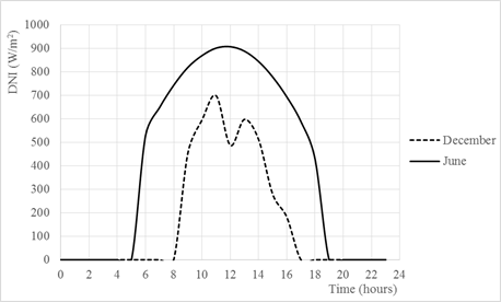
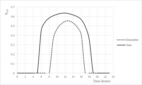
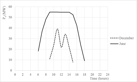
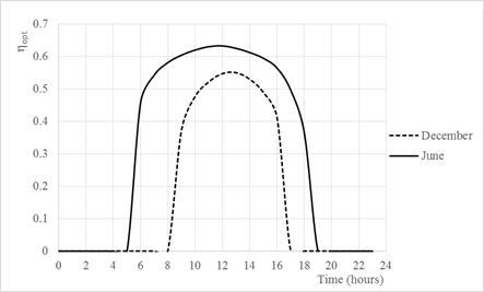
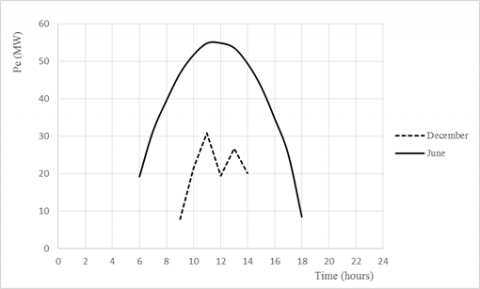
Figures 3-5 show, the time trends of DNI, of optical efficiency of the heliostats field and of net electrical power, for a solar multiple of 1.2, for a clear day in June and an intermediate day in December.
Table 4 shows the annual electricity supplied from the plant, the annual thermal energy supplied to the fluid, the average annual efficiency of field-receiver system, the average efficiency of the power block, the global efficiency of the plant and the load factor CF (percentage of equivalent hours of working at nominal power compared to the total number of hours available in a year), as a function of solar multiple SM.
Figure 3. DNI as a function of time for a clear day in June and an intermediate day in December in Almeria
Figure 4. Heliostat optical efficiency as a function of the time in the Brayton Cycle
Figure 5. Electrical Power as a function of time in the Brayton Cycle plant
Table 4. Annual data of Brayton Cycle Plant
|
SM |
$E_{e l}$ |
$\mathrm{Q}$ |
$\eta_{F R}$ |
$\eta_{P B}$ |
$\eta_{P}$ |
CF (%) |
|
1 |
83751 |
215063 |
0.349 |
0.389 |
0.135 |
19.1 |
|
1.2 |
97943 |
247365 |
0.334 |
0.395 |
0.132 |
22.4 |
|
1.4 |
107812 |
270034 |
0.313 |
0.399 |
0.124 |
24.6 |
|
1.6 |
114535 |
285367 |
0.289 |
0.401 |
0.115 |
26.1 |
|
1.8 |
118057 |
293556 |
0.264 |
0.402 |
0.106 |
27.1 |
|
2.0 |
120297 |
298694 |
0.242 |
0.405 |
0.098 |
27.5 |
2.2 Calculation Model of the combined cycle
Like for the open air Brayton cycle, a similar analysis has been performed for the solar tower power plant with a combined cycle. Table 5 summarizes the design data.
Table 6 provides the values of the air flow rate $(\mathrm{m}),$ of the air temperature at compressor outlet, of the thermal power(Q), of the gas turbine $\left(\eta_{g t}\right)$ and steam turbine efficiencies $\left(\eta_{s t}\right),$ of the net efficiency of the power block $\left(\eta_{P B}\right)$ and of the net electrical power output from the plant, for different outside air temperature and IGV.
By means of the THERMOFLEX code, the following correlations for the exit temperature from the compressor $T_{\text {oc }}$ for the gas turbine efficiency $\eta_{g t}$ and the steam turbine efficiency $\eta_{s t}$ have been developed, considering a variable air flow rate:
for $T_{A}=0^{\circ} \mathrm{C}$,
$T_{o c}=a+\mathrm{b} \cdot x^{3}$
with $\mathrm{a}=246.5919 ; \mathrm{b}=90.25454 ;$ (16)
$\eta_{g t}=a+b / x^{2}$
with $\mathrm{a}=0.308604 ; \mathrm{b}=-3.373074 \cdot 10^{-2}$ (17)
$\eta_{s t}=a+b / x$
with $\mathrm{a}=0.103356 ; \mathrm{b}=-6.824015 \cdot 10^{-2} ;$ (18)
for $T_{A}=25^{\circ} \mathrm{C}$,
$T_{o c}=a \cdot b^{x}$
with $\mathrm{a}=204.3563 ; \mathrm{b}=1.85103 ;$ (19)
$\eta_{g t}=a+b / x^{2}$
with $\mathrm{a}=0.300301 ; \mathrm{b}=-3.125406 \cdot 10^{-2};$ (20)
$\eta_{s t}=a \cdot x^{b}$
with $\mathrm{a}=0.182133 ; \mathrm{b}=-0.414489 ;$ (21)
Table 5. Design data of the Solar Tower Power Plant with Combined Cycle located in Almeria
|
Parameter |
Value |
|
Nominal net electrical Power |
50 MW |
|
Direct Normal Irradiance (DNI) |
850 W/m2 |
|
Zenith angle |
13.850° |
|
Azimuth angle |
-10.713° |
|
Total area of heliostats |
273,784 m2 |
|
Reflectivity of heliostats |
0.94 |
|
Absorptivity of receiver |
0.97 |
|
Optical efficiency of heliostats field |
0.573 |
|
Efficiency of Receiver |
0.835 |
|
Tower height |
105 m |
|
Compressor pressure ratio |
12.5 |
|
Turbine pressure ratio |
8.5 |
|
Net thermodynamic efficiency |
0.449 |
|
Atmospheric air temperature (TA) |
25℃ |
|
gas turbine Inlet air temperature (TIT) |
1000℃ |
|
Mass flow rate |
156 kg/s |
Table 6. Influence of IGV aperture and of inlet air temperature on the performance of the CC plant
|
$T_{A}$ (℃) |
IGV (%) |
M (kg/s) |
T (℃) |
Q (MW) |
$\eta_{g t}$ |
$\eta_{s t}$qq |
$\eta_{P B}$ |
$P_{e l}$ (MW) |
|
0 |
100 |
168 |
359 |
122 |
0.275 |
0.167 |
0.442 |
53.8 |
|
0 |
80 |
137 |
307 |
107 |
0.271 |
0.181 |
0.452 |
48.2 |
|
0 |
60 |
103 |
272 |
84 |
0.229 |
0.207 |
0.436 |
37 |
|
25 |
100 |
156 |
378 |
111 |
0.268 |
0.182 |
0.450 |
50 |
|
25 |
80 |
125 |
335 |
95 |
0.253 |
0.200 |
0.453 |
43 |
|
25 |
60 |
94 |
296 |
76 |
0.213 |
0.225 |
0.438 |
33 |
|
50 |
100 |
139 |
389 |
101 |
0.256 |
0.203 |
0.460 |
46 |
|
50 |
80 |
112 |
358 |
85 |
0.227 |
0.224 |
0.452 |
38 |
|
50 |
60 |
84 |
330 |
67 |
0.174 |
0.251 |
0.426 |
28 |
for $T_{A}=50^{\circ} \mathrm{C}$,
$T_{o c}=a \cdot b^{x}$
with a $=255.1888 ; \mathrm{b}=1.60495$ (22)
$\eta_{g t}=a+b / x$
with $\mathrm{a}=0.38281 ; \mathrm{b}=-0.112634$ (23)
$\begin{array}{c}\eta_{s t}=a \cdot b^{x} \\ \text { with } \mathrm{a}=0.347898 ; \mathrm{b}=-0.545025\end{array}$ (24)
For a constant flow rate operation and variable TIT the following correlations were obtained:
for $T_{A}=0^{\circ} C$,
$T I T=a \cdot Q^{3}+\cdot Q^{2}+c \cdot Q+d$
with $a=5.898722 \cdot 10^{-5} ; \mathrm{b}=-2.019249 \cdot 10^{-2}$
$\mathrm{c}=10.918839 ; \mathrm{d}=190.248464$ (25)
$\eta_{g t}=a+b \cdot T I T^{0.5}+c / T I T^{1.5}$
with $a=0.326549 ; \mathrm{b}=-1.445094 \cdot 10^{-7} ;$
$\mathrm{c}=-3228.2688 ;$ (26)
$\eta_{s t}=a \cdot T I T^{3}+b \cdot T I T^{2}+c \cdot T I T+d$
with $a=8.33333 \cdot 10^{-11} ; b=-6.214285 \cdot 10^{-7} ;$
$c=10.918839 \cdot 10^{-3} ; d=-0.296885$ (27)
for $T_{A}=25^{\circ} \mathrm{C}$,
$T I T=a \cdot Q^{3}+b \cdot Q^{2}+c \cdot Q+d$
with $a=7.86633 \cdot 10^{-5} ; b=-2.38838 \cdot 10^{-2}$;
$c=11.733322 ; \mathrm{d}=214.908106$ (28)
$\eta_{g t}=a+b \cdot T I T+c / T I T^{1.5}$
with a $=0.323386 ; \mathrm{b}=-7.309416 \cdot 10^{-6} ;$
$\mathrm{c}=-3214.9926$ (29)
$\eta_{s t}=a+b \cdot T I T^{2}+c \cdot T I T^{0.5}$
with a $=-0.480034 ; \mathrm{b}=-1.443485 \cdot 10^{-7} ;$
$\mathrm{c}=2.629234 \cdot 10^{-2}$ (30)
for $T_{A}=50^{\circ} \mathrm{C}$,
$T I T=a+b \cdot x^{0.5}+c / x^{0.5}$
with $a=-1013.990342 ; \mathrm{b}=205.346943 ;$
$\mathrm{c}=2663.537571$ (31)
$\eta_{g t}=a+b \cdot T I T^{0.5}+c / T I T^{2}$
with a $=0.147127 ; \mathrm{b}=3.3784093 \cdot 10^{-3}$;
$\mathrm{c}=-66915.18$ (32)
$\eta_{s t}=a \cdot T I T^{2}+b \cdot T I T+c$
with $a=-0.0000003 ; \mathrm{b}=-6.99999 \cdot 10^{-4} ; \mathrm{c}=-0.149$ (33)
All above correlations have a correlation coefficient of 99.99% and a maximum error less than 0.5%.
The maximum thermal power transmitted from the receiver to the power block, in this plant, is 122 MW.
Using DELSOL-3 code, the total area of the heliostats $A_{e}$, for SM = 1, in the design conditions of Table 5, resulted to be 273,784 $m^{2}$; the height of the tower and the size of the receiver resulted equal to those of the Brayton cycle plant.
The values of the optical efficiency, calculated by DELSOL-3 code for SM = 1.2, as a function of the zenith and azimuth angle of the sun, are given in Table 7.
Table 7. Optical efficiency of the solar field of the Combined Cycle Plant for SM=1.2 as a function of sun zenith and azimuth angles
|
|
0.5 |
7 |
15 |
30 |
45 |
60 |
75 |
85 |
90 |
|
0 |
0.641 |
0.641 |
0.649 |
0.655 |
0.661 |
0.658 |
0.635 |
0.521 |
0.305 |
|
30 |
0.641 |
0.65 |
0.658 |
0.667 |
0.668 |
0.648 |
0.532 |
0.296 |
0.214 |
|
60 |
0.641 |
0.648 |
0.654 |
0.66 |
0.657 |
0.633 |
0.518 |
0.288 |
0.211 |
|
90 |
0.64 |
0.644 |
0.645 |
0.64 |
0.628 |
0.596 |
0.478 |
0.253 |
0.178 |
|
120 |
0.64 |
0.638 |
0.633 |
0.615 |
0.59 |
0.548 |
0.428 |
0.238 |
0.175 |
|
150 |
0.64 |
0.633 |
0.62 |
0.591 |
0.555 |
0.505 |
0.391 |
0.221 |
0.164 |
|
180 |
0.639 |
0.629 |
0.612 |
0.574 |
0.531 |
0.475 |
0.362 |
0.205 |
0.156 |
|
210 |
0.639 |
0.627 |
0.609 |
0.568 |
0.523 |
0.464 |
0.35 |
0.194 |
0.145 |
|
240 |
0.639 |
0.629 |
0.612 |
0.575 |
0.533 |
0.477 |
0.364 |
0.207 |
0.157 |
|
270 |
0.64 |
0.633 |
0.622 |
0.593 |
0.558 |
0.508 |
0.393 |
0.227 |
0.172 |
|
300 |
0.64 |
0.639 |
0.634 |
0.617 |
0.593 |
0.551 |
0.432 |
0.249 |
0.191 |
|
330 |
0.641 |
0.645 |
0.646 |
0.642 |
0.63 |
0.598 |
0.482 |
0.285 |
0.222 |
Figures 6-7 show the optical efficiency of the heliostats field and the net electrical power as functions of time for the same value of the solar multiple, for a clear day in June and an intermediate day in December.
Figure 6. Heliostat optical efficiency as a function of time in the Combined Cycle plant
Figure 7. Electrical power as a function of time in the Combined Cycle plant
Table 8 shows the annual electricity $\left(E_{e l}\right)$ supplied by the plant and the thermal energy (Q) supplied to the fluid, the average annual values of the field-receiver system efficiency $\left(\eta_{F R}\right),$ the efficiency of the power block $\left(\eta_{P B}\right),$ the global efficiency $\left(\eta_{P}\right)$ and the capacity factor CF as functions of the solar multiple SM.
Table 8. Annual data of CC Plant
|
SM |
$E_{e l}$ |
$\mathrm{Q}$ |
$\eta_{F R}$ |
$\eta_{P B}$ |
$\eta_{P}$ |
CF (%) |
|
1 |
95411 |
227627 |
0.419 |
0.408 |
0.171 |
21.7 |
|
1.2 |
109538 |
253602 |
0.379 |
0.431 |
0.163 |
25.0 |
|
1.4 |
121638 |
276993 |
0.355 |
0.439 |
0.156 |
27.7 |
|
1.6 |
127156 |
287877 |
0.322 |
0.441 |
0.142 |
29.0 |
|
1.8 |
134293 |
301372 |
0.300 |
0.445 |
0.134 |
30.6 |
|
2.0 |
137408 |
306415 |
0.275 |
0.448 |
0.123 |
31.4 |
The performance of a 50 MW solar plant with molten salts have been determined using the SAM code [36]. This represents the most common type of solar tower power plant. Hence, it has been analyzed and considered as a reference case.
In design conditions, with a minimum and maximum salts temperature of 290℃ and 565℃, the heliostats area is 247,499 $m^{2}$, the height of the tower 93.3 m, the diameter of the receiver 8 m and its height 8.53 m.
Table 9 shows the annual values of the electricity produced $\left(E_{e l}\right),$ the thermal energy (Q) transferred to the fluid in the receiver, the receiver-field efficiency $\left(\eta_{F R}\right),$ the efficiency of the power block $\left(\eta_{P B}\right),$ the overall efficiency of the system $\left(\eta_{P}\right)$ and the capacity factor as functions of the solar multiple.
Table 9. Annual data of Molten Salts Plant
|
SM |
$E_{e l}$ |
$\mathrm{Q}$ |
$\eta_{F R}$ |
$\eta_{P B}$ |
$\eta_{P}$ |
CF (%) |
|
1 |
61022 |
209000 |
0.415 |
0.292 |
0.121 |
13.9 |
|
1.2 |
77424 |
253602 |
0.396 |
0.305 |
0.120 |
17.7 |
|
1.4 |
88554 |
285000 |
0.385 |
0.310 |
0.119 |
20.2 |
|
1.6 |
96011 |
305000 |
0.358 |
0.315 |
0.112 |
21.9 |
|
1.8 |
101201 |
330000 |
0.345 |
0.306 |
0.105 |
23.1 |
|
2.0 |
102255 |
330000 |
0.320 |
0.309 |
0.098 |
23.3 |
To establish the economic convenience of the two solar plants, the calculation of the levelized cost of energy LCOE ($/kWh) was carried out, utilizing the NREL algorithm [37].
LCOE is defined as [37, 38]:
$L C O E=\frac{\text {Capital cost} \cdot \mathrm{CRF}+\text {Fixed } \text { O&M cost }}{8760 \cdot \mathrm{CF}}$$+ Variable O\&M Cost$ (34)
Being
$C R F=\frac{i(1+i)^{n}}{(1+i)^{n}-1}$ (35)
In Eq. (34) Capital Cost is the unit power cost (\$/kW) of the plant, Fixed O&M Cost represents the fixed operation and maintenance cost in a year (\$/kWy), Variable O&M Cost is the variable operation and maintenance cost (\$/kWh), CF is the capacity factor and 8760 is the number of hours in a year.
In Eq. (35) i is the discount rate and n the lifetime of the plant in years.
The values of above data assumed in our calculations, with the exception of the Capital Cost, are reported in Table 10.
Table 10. Cost data for the economic analysis
|
Lifetime (years) |
25 |
|
Discount rate |
4% |
|
Specific cost of heliostats |
200 \$/m2 |
|
Specific cost of Receiver |
122 \$/m2 |
|
Specific cost of CC Power Block & Balance of plant |
1500\$/kW |
|
Specific cost of Brayton Cycle Power Block & Balance of plant |
850 \$/kW |
|
Specific cost of Molten salts Power Block & Balance of plant |
940 \$/kW |
|
Fixed O&M Cost |
27.5 \$/kW y |
|
Variable O&M Cost |
0.003 \$/kWh |
|
Electricity Price |
12 cent \$/kWh |
|
Electricity Cost Escalation rate |
2% |
Table 11. Costs of Brayton Cycle Plant and LCOE
|
SM |
1 |
1.2 |
1.4 |
1.6 |
1.8 |
2.0 |
|
Ground Cost (M\$) |
14.5 |
15.97 |
17.64 |
20.0 |
21.85 |
24.07 |
|
Heliostats Cost (M\$) |
60.49 |
69.46 |
79.62 |
93.92 |
106.2 |
118.7 |
|
Receiver Cost (M\$) |
18.37 |
26.47 |
36.06 |
47.1 |
59.18 |
73.6 |
|
Tower Cost (M\$) |
1.58 |
1.92 |
2.42 |
2.87 |
3.46 |
4.29 |
|
Total Cost (M\$) |
137.4 |
156.3 |
178.2 |
206.4 |
232.2 |
263.2 |
|
Unit Capital Cost \$/kW |
2748 |
3126 |
3564 |
4123 |
4643 |
5263 |
|
LCOE cent \$/kWh |
12.4 |
11.9 |
12.2 |
13.0 |
14.0 |
15.4 |
Table 12. Costs of CC Plant and LCOE
|
SM |
1 |
1.2 |
1.4 |
1.6 |
1.8 |
2.0 |
|
Ground Cost (M\$) |
13.56 |
14.82 |
16.7 |
18.11 |
20.52 |
22.63 |
|
Heliostats Cost (M\$) |
54.75 |
62.48 |
73.9 |
82.45 |
97.13 |
109.9 |
|
Receiver Cost (M\$) |
18.37 |
26.47 |
36.06 |
47.1 |
59.18 |
73.6 |
|
Tower Cost (M\$) |
1.57 |
1.93 |
2.42 |
2.87 |
3.46 |
4.29 |
|
Total Cost (M\$) |
163.2 |
180.7 |
204.1 |
225.5 |
255.3 |
285.4 |
|
Unit Capital Cost \$/kW |
3265 |
3613 |
4081 |
4510 |
5105 |
5708 |
|
LCOE cent \$/kWh |
12.7 |
12.1 |
12.2 |
12.7 |
13.5 |
14.6 |
Table 13. Costs of Molten Salts Plant and LCOE
|
SM |
1 |
1.2 |
1.4 |
1.6 |
1.8 |
2.0 |
|
Ground Cost (M\$) |
12.69 |
14.60 |
16.52 |
18.29 |
20.01 |
21.15 |
|
Heliostats Cost (M\$) |
49.49 |
61.13 |
72.88 |
83.57 |
94.35 |
100.9 |
|
Receiver Cost (M\$) |
26.15 |
29.92 |
32.29 |
37.68 |
42.18 |
48.45 |
|
Tower Cost (M\$) |
1.40 |
1.50 |
1.60 |
1.74 |
1.83 |
2.21 |
|
Total Cost (M\$) |
136.7 |
154.2 |
170.3 |
182.7 |
205.2 |
218.8 |
|
Unit Capital Cost \$/kW |
2734 |
3083 |
3405 |
3765 |
4104 |
4376 |
|
LCOE cent \$/kWh |
16.9 |
14.8 |
14.2 |
14.3 |
14.6 |
15.3 |
Table 11 shows the costs for the ground, the heliostats, the receiver, the tower and the total cost, the Capital Cost and the LCOE values, for the Brayton plant, at varying of solar multiple, evaluated by Eq. (34) and (35).
Table 12 reports the same data for the combined cycle plant, while Table 13 refers to the molten salts reference plant.
To obtain the Capital Cost values, the total costs of the plants were obtained as the sum of the cost of the ground, of the heliostats, the price of the receiver and of the power block.
The following assumptions were made [39, 40]:
Occupied ground area: $(\left.A_{e}=1.3+0.18\right) \mathrm{km}^{2}$
Ground cost (land cost and construction costs for building and roads): $25.3 \$ / m^{2}$ The tower cost (\$) was calculated by the following formula:
$C_{T}=552,000 \cdot e^{H / 100}$ (36)
where, H is the height of the tower in meters.
Power Block costs:
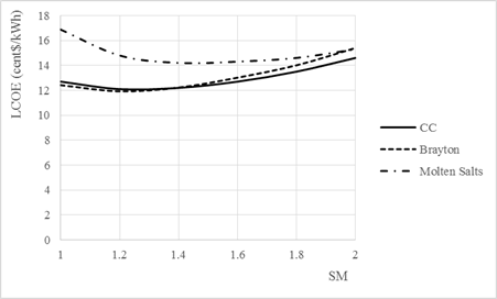
Tables 1 and 2, containing the design data of the two systems, show that a 50 MW electrical power plant can be obtained, in the case of the combined cycle, with a heliostats area of 273,784 $m^{2}$, against an area of 302,499 $m^{2}$ in the case of the Brayton cycle, with a reduction of 11%. This is mainly due to the difference between the thermodynamic net efficiency of the power block, which is 0.449 in the combined cycle and 0.404 in the Brayton cycle. Figure 8 shows the comparison of LCOE as function of solar multiple for the three plants.
Figure 8. Levelized Cost of Energy (LCOE) as a function of solar multiple (SM)
The comparison of Tables 4 and 9, showing the annual values of the quantities of interest for the two systems, indicates, for a 1.2 solar multiple (for which there is the minimum value of LCOE), that the annual electricity supplied by the combined cycle is 109,538 MWh, against a value of 97,943 MWh in the Brayton cycle, with an increase of about 12%. The capacity factor is 25% in the combined cycle, compared with 22.4% of the Brayton cycle. The average annual plant efficiency is 16.3% in the combined cycle against the 13.2% of the Brayton cycle
The 50 MW plant using molten salts, with an area of heliostats of 247,497 $m^{2}$ (lower than both the Brayton plant and the combined Brayton cycle due to the smaller radiative losses from the receiver), provides an annual electrical energy of 61,022 MWh for SM = 1, as shown in Table 9. Figure 9 shows the annual energy per square meter obtained with the three systems, as a function of the solar multiple. The graph shows that the maximum value is obtained for SM = 1.2 and is 0.282 $\mathrm{MWh} / \mathrm{m}^{2}$ for the Brayton plant, 0.351 $\mathrm{MWh} / \mathrm{m}^{2}$ for the combined cycle plant and 0.253 $\mathrm{MWh} / \mathrm{m}^{2}$ for the plant using molten salts. Therefore, the specific energy of the Brayton plant is 11.5% greater than that obtained for the plant using molten salts, while for the combined cycle there is an increase of 38.7% with respect to the system using molten salts.
Figure 9. Annual Electrical Energy per square meter of heliostat as a function of solar multiple
Based on these results, it is evident that the technical performance of the combined cycle is superior to that of the Brayton cycle, and both of these systems have better performances than the plant using molten salts. For the value of the solar multiple of 1.2, the cost of the Brayton plant is lower (156.32 M\$) than that of the combined cycle (180.7 M\$), while the cost of the molten salt plant resulted as 154.2 M\$. Unit cost values were, respectively, 3126 \$/kW, 3613 \$/kW and 3083 \$/kW. The capacity factor of the plant using molten salts resulted at 17.67% (against the values of 22.4 and 25%), for the same value of the solar multiple. The cost of electricity (LCOE) produced over the life of the plants, see Tables 10 and 11, resulted 11.9 cent\$/ kWh for the Brayton cycle and 12.1 cent\$/ kWh for the combined cycle, with a slight economic advantage for the Brayton cycle.
The economical convenience of both plants is greater than that of molten salt systems, see Figure 8, which shows that the cost of electricity produced by a molten salt system presents a minimum value close to 14 cent\$/ kWh.
A calculation method was developed for the design and the estimation of the annual performance of two 50 MWe concentrating solar tower power plants that use atmospheric air as heat transfer fluid. In the first plant the air evolves in an open Brayton cycle; the second plant is a combined cycle. The annual performance of the two systems has been estimated, in terms of electricity, average annual efficiency of the heliostats field-receiver system, efficiency of the thermodynamic cycle and of the entire plant, comparing these parameters with those of a plant with molten salts of the same nominal power output. The technical-economic performance of the two proposed systems is superior to molten salt systems, currently widely established on a global scale. In fact, the specific annual electrical energy (per square meter of heliostat) is, in the Brayton cycle, 11.5% higher than that obtained with the system using molten salts, while in the combined cycle plant an increase of 38% was achieved. The cost of electricity, in terms of LCOE, amounted to 11.9 cent\$/kWh for the Brayton cycle, to 12.1 cent\$/kWh for combined cycle, against the value of 14 cent\$/kWh for the reference molten salts plant, with savings of 15% and 13.6%.
|
A |
area, m2 |
|
CF |
capacity factor, - |
|
CRF |
cost recovery factor, - |
|
DNI E |
direct normal irradiance, W. m-2 annual energy, MWh |
|
H |
enthalpy, kJ/kg |
|
h |
heat transfer coefficient, W.m-2.K-1 |
|
i |
discount rate, - |
|
LCOE |
levelized cost of electricity, $/kWh |
|
m |
mass flow rate, kg.s-1 |
|
n |
lifetime of the plant, years |
|
P |
power, MW |
|
Q |
thermal power, MW |
|
SM |
solar multiple, - |
|
T |
temperature, ℃ |
|
TIT |
turbine inlet temperature, ℃ |
|
x |
dimensionless mass flow rate, - |
|
Greek symbols |
|
|
$\varepsilon$ |
emissivity, - |
|
$\eta$ |
efficiency, - |
|
$\sigma$ |
Stephan Boltzman Constant, W/m2 K4 |
|
Subscripts |
|
|
A |
air |
|
c |
compressor |
|
con |
convective |
|
e |
heliostat |
|
el |
electrical |
|
gt |
gas turbine |
|
o |
outlet |
|
opt |
optical |
|
r |
regenerator |
|
rad |
radiative |
|
R |
receiver |
|
st |
steam turbine |
[1] Ferraro, V., Marinelli, V., Settino, J., Nicoletti, F. (2020). A calculation method to estimate the thermodynamic performance of solar tower power plants with an open air Brayton cycle and a combined cycle. TECNICA ITALIANA-Italian Journal of Engineering Science, 64(2-4): 268-276. https://doi.org/10.18280/ti-ijes.642-422
[2] Bruno, R., Bevilacqua, P., Longo, L., Arcuri, N. (2015). Small size single-axis PV trackers: Control strategies and system layout for energy optimization. Energy Procedia, 82: 737-743. https://doi.org/10.1016/j.egypro.2015.11.802
[3] Falcone, P. (1986). A handbook for solar central receiver design. SANDIA National Laboratories. https://doi.org/10.2172/6545992
[4] Romero-Alvarez, M. (2007). Concentrating Solar Thermal Power- Handbook of Energy Efficiency and Renewable Energy. Plataforma Solar de Almeria. CIEMAT.
[5] Siva Reddy, V., Kaushik, S.C., Ranjan, K.R., Tyagi, S.K. (2013). State-of-the-art of solar thermal power plants - A review. Renewable and Sustainable Energy Reviews, 27: 258-273. https://doi.org/10.1016/j.rser.2013.06.037
[6] Xu, X., Vignarooban, K., Xu, B., Hsu, K., Kannan, A.M. (2016). Prospects and problems of concentrating solar power technologies for power generation in the desert regions. Renewable and Sustainable Energy Reviews, 53: 1106-1131. https://doi.org/10.1016/j.rser.2015.09.015
[7] Boretti, A., Castelletto, S., Al-Zubaidy, S. (2019). Concentrating solar power tower technology: Present status and outlook. Nonlinear Engineering, 8(1): 10-31. https://doi.org/10.1515/nleng-2017-0171
[8] Maccari, A., Buono, S., Maciocco, L. (2001). Solar Thermal Energy Production. Guidelines and future programs of ENEA, ENEA/TM/PRES/2001_07. Available at: www.enea.it/com/ing, accessed on 12 June 2001.
[9] Ortega, J.I., Burgaleta, J.I., Tellez, F. (2008). Central receiver system solar plant using molten salt as heat transfer fluid. Journal of Solar Energy Engineering, 130(2): 1-6. https://doi.org/10.1115/1.2807210
[10] Rodriguez, M.M., Marquez, J.M., Biencinto, M., Adler, J.P., Diez, L.E. (2009). First experimental results of a solar PTC facility using gas as the heat transfer fluid. 5th International Symposium on Concentrated Solar Power and Chemical Energy, Berlin, Germany.
[11] Chacartegui, R., Munoz de Escalona, J.M., Sanchez, D., Monje, B., Sanchez, T. (2011). Alternative cycles based on carbon dioxide for central receiver solar power plants. Applied Thermal Engineering, 31: 872-879. https://doi.org/10.1016/j.applthermaleng.2010.11.008
[12] Al-Sulaiman, F.A., Atif, M. (2015). Performance comparison of different supercritical carbon dioxide Brayton Cycles integrated with a solar power tower. Energy, 82: 61-71. https://doi.org/10.1016/j.energy.2014.12.070
[13] Vasquez Padilla, R., Soo Too, Y.C., Benito, R., Stein, W. (2015). Exergetic analysis of supercritical Brayton cycles integrated with solar receivers. Applied Energy, 148: 348-365. https://doi.org/10.1016/j.apenergy.2015.03.090
[14] Kumar, P., Srinivasan, K. (2016). Carbon dioxide based power generation in renewable energy systems. Applied Thermal Engineering, 109: 831-840. https://doi.org/10.1016/j.applthermaleng.2016.06.082
[15] de Araujo Passos, L.A., de Abreu, S.L., da Silva, A.K. (2017). Optimal scale of solar-trough powered plants operating with carbon dioxide. Applied Thermal Engineering, 124: 1203-1212. https://doi.org/10.1016/j.applthermaleng.2017.06.004
[16] Reyes-Belmonte, M.A., Sebastiàn, A., Gonzàlez-Aguilar, J., Romero, M. (2017). Performance comparison of different thermodynamic cycles for an innovative central receiver solar power plant. AIP Conference Proceedings, 1850(1): 160024. https://doi.org/10.1063/1.4984558
[17] Ferraro, V., Marinelli, V. (2012). An evaluation of thermodynamic solar plants with cylindrical parabolic collectors and air turbine engines with open Joule-Brayton cycle. Energy, 44(1): 862-869. https://doi.org/10.1016/j.energy.2012.05.005
[18] Ferraro, V., Imineo, F., Marinelli, V. (2013). An improved model to evaluate thermodynamic solar plants with cylindrical parabolic collectors and air turbine engines in open Joule-Brayton cycle. Energy, 53: 323-331. https://doi.org/10.1016/j.energy.2013.02.051
[19] Amelio, M., Ferraro, V., Marinelli, V., Summaria, A. (2014). An evaluation of the performance of an integrated combined solar plant provided with an air-linear parabolic collectors. Energy, 69: 742-748. https://doi.org/10.1016/j.energy.2014.03.068
[20] Rovense, F., Amelio, M., Ferraro, V., Scornaienchi, Analysis of a concentrating solar power tower operating with a close Joule Brayton cycle and thermal storage. International Journal of Heat and Technology, 34(3): 485-490. https://doi.org/10.18280/ijht.340319
[21] Heller, P., Pfander, M., Denk, T., Tellez, F., Valverde, A., Fernandez, J., Ring, A. (2006). Test and evaluation of a solar powered gas turbine system. Solar Energy, 80(10): 1225-1230. https://doi.org/10.1016/j.solener.2005.04.020
[22] https://www.csiro.au/en/Research/EF/Areas/Renewable-and-low-emission-tech/Solar-energy/Solar-thermal/, accessed on Jun. 31, 2020.
[23] Nakatani, H., Obada, T., Kobayashi, K., Watabe, M., Tagawa, M. (2012). Development of a concentrated solar power generation system with a hot-air turbine. Mitsubishi Heavy Industries Technical Review, 49(1): 1-5.
[24] (2014). Solar Air Turbine Project Final report: project results, CSIRO, Commonwealth Scientific Industrial Research Organisation, March 2014
[25] Quero, M., Korzynietz, R., Ebert, M., Jiménez, A.A., del Río, A., Brioso, J.A. (2014). Solugas – Operation experience of the first solar hybrid gas turbine system at MW scale. Energy Procedia, 49: 1820-1830. https://doi.org/10.1016/j.egypro.2014.03.193
[26] Korzynietz, R., Brioso, J.A., del Río, A., Quero, M., Gallas, M., Uhlig, R., Ebert, M., Buck, R., Teraji, D. (2016). Solugas – Comprehensive analysis of the solar hybrid Brayton plant. Solar Energy, 135: 578-589. https://doi.org/10.1016/j.solener.2016.06.020
[27] Spelling, J., Favrat, D., Martin, A., Agsburger, G. (2012). Thermoeconomic optimization of a combined-cycle solar tower power plant. Energy, 41(1): 113-120. https://doi.org/10.1016/j.energy.2011.03.073
[28] Spelling J, Laumert B, Fransson T. (2014). Advanced hybrid solar tower combined-cycle power plants. Energy Procedia, 49: 1207-1217. https://doi.org/10.1016/j.egypro.2014.03.130
[29] Okoroigwe E, Madhlopa A. (2016). An integrated combined cycle system driven by a solar tower: A review. Renewable and Sustainable Energy Reviews, 57: 337-350. https://doi.org/10.1016/j.rser.2015.12.092
[30] Rovira, A., Sànchez, C., Valdés, M., Abbas, R., Barbero, R., Montes, M.J., Muñoz, M., Muñoz-Antòn, J., Ortega, G., Varela, F. (2018). Comparison of different technologies for integrated solar combined cycles: Analysis of concentrating technology and solar integration. Energies, 11(5): 1-16.
[31] Amani, M., Ghenaiet, A., Smaili, A. (2018). Determination of the performance of a solar tower integrated with a combined cycle. 2018 6th International Renewable and Sustainable Energy Conference (IRSEC), Rabat, Morocco, pp. 1-6. https://doi.org/10.1109/IRSEC.2018.8703000
[32] Thermoflow Inc. Southborough (USA) -Thermoflex Program, version 22.0.1. https://www.thermoflow.com/, accessed on Mar. 01, 2020.
[33] Oakdale Engineering - Datafit program, version 8.1.69. https://download.cnet.com/developer/oakdale-engineering/i-52716/, accessed on Feb. 01, 2020.
[34] Eddhibi, F., Amara, M.B., Balghouthi, M., Guizani, A. (2015). Optical study of solar tower power plants. Tunisia-Japan Symposium: R&D of Energy and Material Sciences IOP Publishing Journal of Physics: Conference Series, 596.
[35] WinDelsol 1.0 User Guide. (2002). Aicia - Ciemat - Solucar, Central Receiver Technologies, Madrid, Spain.
[36] Solar Advisor Model reference manual for CSP trough systems SAM version 3.0. (2009). National Renewable Energy Laboratory. Golden, Colorado, USA.
[37] Levelized Cost of Energy Calculator. https://www.nrel.gov/analysis/tech-lcoe.html accessed on Jun. 30, 2020.
[38] Short, W., Packey, D.J., Holt, T. (1995). A Manual for the Economic Evaluation of Energy Efficiency and Renewable Energy Technologies. NREL/TP-462-5173.
[39] Zhang, W. (2009). Concentrating solar power - state of the art, cost analysis and pre-feasibility study for the implementation in China. Diplomarbeit, Institut für Energiewirtschaft und Rationelle Energieanwendung, IER, Stuttgart (Germany).
[40] Kolb, G.J., Ho, C.K., Mancini, T.R., Gary, J.A. (2011). Power tower technology roadmap and cost reduction plan. SANDIA REPORT SAND2011-2419.
[41] Lozza, G. (2006). Gas Turbines and Combined Cycles. Soc.Ed. Esculapio, Bologna, Italy.