Bayo Johnson Akinbo* | Bakai Ishola Olajuwon
© 2020 IIETA. This article is published by IIETA and is licensed under the CC BY 4.0 license (http://creativecommons.org/licenses/by/4.0/).
OPEN ACCESS
In this paper, analyses of the thermal and thermo diffusion effects on the Heat and Mass transfer in a Viscous Fluid over an exponential stretching Surface in the presence of heat absorption have been investigated. The two-dimensional boundary-layer equations governing the system is obtained in form of partial differential equations by Boussinesq approximation and transformed into a system of the ordinary differential equation via similarity variables. The resulting equations are then solved, using Homotopy Analysis Method and the effect of heat absorption, radiation parameter and other parameters encountered are presented graphically and discussed, while the effect of Local skin-friction, Nusselt and Sherwood numbers are presented numerically. The result shows among other results obtained that the effect of Lorentz force on velocity acts against the fluid flow, thereby resist the motion of the fluid of which its aftermath reduces the fluid velocity while its temperature improves due to the frictional heating generated across the boundary layer.
similarity variable, magnetic field, heat absorption, heat and mass transfer, homotopy analysis method (HAM)
The dynamics of heat and mass transfer over a stretching surface has wide application in many manufacturing industries and technological process among which are paper production, glass-fiber production, hot metal rolling, plastic sheet and drawing of plastic films e.t.c. An early investigation are carried out by Sakiadis et al. [1-3] and based on the foregoing application, it has attracted the attention of many researchers and extensively studied in the literature. Anuar [4] studied MHD boundary layer flow due to an exponentially stretching sheet with radiation effect. Seini and Makinde [5] buttressed the work of Anuar [4] to include chemical reaction which was solved numerically using the fourth-order Runge-Kutta integration scheme with a modified version New-Raphson algorithms. The results obtained agreed with the previous work done in the literature where the surface shear stress increases with increasing magnetic parameter whilst the transfer rate increases with Prandtl number. Other authors like Partha et al. [6], Sajid and Hayat [7], Noran et al. [8], Yasir et al. [9], Bidin and Nazar [10], Devi et al. [11], Jat and Gopi [12] and Chen [13] worked on exponential stretching sheet or surface with different conditions and their result agreed with other results in the literature.
In addition to the foregoing contribution of authors, the inclusion of porosity term has not been left out. Nagbhoohan et al. [14] included porosity term in their investigation while studying flow and heat transfer over an exponential gradient dependent heat sink and thermal radiation. The magnetic field reduces the heat transfer rate, which in turn improves the temperature with the boundary layer according to Animasaun et al. [15] while investigating the Casson fluid flow with variable thermo-physical property along exponentially stretching sheet with suction and exponentially decaying internal heat generation, using the Homotopy Analysis Method. Heat transfer and boundary layer flow past a stretching porous wall with temperature gradient dependent heat sink was investigated by Singh [16] while Mukhopadhyay et al. [17] studied mass transfer over an exponentially stretching porous sheet embedded in a stratified medium. Due to the destructive chemical reaction, the result shows among others that the solute boundary layer becomes thinner and for constructive chemical reaction, it becomes thicker. Other researchers like; Bhattacharyya and Layek [18], Chauham and Onkha [19], Cortell [20] included porosity term in their investigation.
Motivated by the previous work done in the literature, this present investigation is to extend the work in Seine and Makinde [5] to include thermal and thermo diffusion effects on the heat and mass transfer in a viscous fluid over an exponentially stretching surface in the presence of heat sink. The governing equations are solved analytically using Homotopy Analysis Method (HAM) developed by Liao [21, 22] and the effects of the different parameter on fluid flow are discussed numerically and graphically.
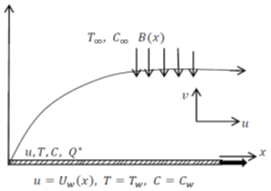
Consider a steady-state, incompressible two-dimensional boundary layer flow with heat and mass transfer of a viscous and electrically conducting fluid induced by a stretching surface and is placed in a quiescent fluid of the ambient temperature $T_{\infty}$ and concentration $C_{\infty}$. The variable magnetic field B(x) is applied normal to the sheet and the magnetic Reynolds number is assumed to be small and so, the induced magnetic field is neglected. The reaction rate is taken as R while the heat absorption coefficient is Q* (See Figure 1). In view of the assumption mention above and usual Boussinesq’s approximation, the geometry and governing equations of this present problem can be expressed as:
Figure 1. Flow configuration and coordinate system
Continuity Equation:
$\frac{\partial u}{\partial x}+\frac{\partial v}{\partial y}=0$ (1)
Momentum Equation:
$u \frac{\partial u}{\partial x}+v \frac{\partial u}{\partial y}=v \frac{\partial^{2} u}{\partial y^{2}}-\frac{\sigma B^{2}}{\rho} u$ (2)
Energy Equation:
$u \frac{\partial T}{\partial x}+v \frac{\partial T}{\partial y}=\frac{k}{\rho C_{p}} \frac{\partial^{2} T}{\partial y^{2}}-\frac{1}{\rho C_{p}} \frac{\partial q_{r}}{\partial y}+\frac{v}{C_{p}}\left(\frac{\partial u}{\partial y}\right)^{2}$
$+\frac{\sigma B^{2}}{\rho C_{p}} u^{2}+\frac{D_{m} K_{T}}{C_{s} C_{p}} \frac{\partial^{2} C}{\partial y^{2}}+\frac{Q^{*}\left(T-T_{\infty}\right)}{\rho C_{p}}$ (3)
Concentration equation:
$u \frac{\partial C}{\partial x}+v \frac{\partial C}{\partial y}=D_{m} \frac{\partial^{2} C}{\partial y^{2}}+\frac{D_{m} K_{T}}{T_{m}} \frac{\partial^{2} T}{\partial y^{2}}-R\left(C-C_{\infty}\right)$ (4)
where, u and v respectively denote the velocity components in x and y directions, v is the kinematic viscosity, $\rho$ is the fluid density, k is the thermal conductivity, Cp is the specific heat at constant pressure, Dm is the mass diffusivity coefficient, qr is the radiative heat flux, R is the reaction rate parameter, Q* is the heat source\absorption coefficient, Tm is the mean fluid temperature while T and C respectively denote the fluid temperature and concentration.
The corresponding boundary conditions for this present investigation are:
$u=U_{w}=U_{0} e^{x / L}, \quad v=0$
$T=T_{w}=T_{\infty}+T_{0} e^{x /(2 L)}$
$C=C_{w}=C_{\infty}+C_{0} e^{x /(2 L)} \quad$ at $y=0$
$u \rightarrow 0, \quad T \rightarrow T_{\infty}, \quad C \rightarrow C_{\infty}$ as $y \rightarrow \infty$ (5)
Which agreed with Anuar [4] and Seini and Makinde [5]. where, T0 and C0 are respectively taken as reference temperature and reference concentration while L is the reference length. The radiative heat flux is simplified by Rosseland approximation as:
$q_{r}=\frac{-4 \sigma^{*}}{3 k^{*}} \frac{\partial T^{4}}{\partial y}$ (6)
where, $\sigma^{*}$ is the sterfan-Boltzmann constant and k* is the mean of the absorption coefficient. Following Hossain et al. [23] this approximation is valid at points optically far from the boundary surface and is good only for intensive absorption for an optically thick boundary layer. It is assumed that the temperature differences within the flow are such that the term T4 can be expressed as a linear function of temperature by expanding T4 in a Taylor series about $T_{\infty}$ as:
$T^{4}=T_{\infty}^{4}+4 T_{\infty}^{3}\left(T-T_{\infty}\right)+6 T_{\infty}^{2}\left(T-T_{\infty}\right)^{2}+\ldots$ (7)
and neglecting the higher-order terms beyond the first degree in $\left(T-T_{\infty}\right)$ gives:
$T^{4} \approx 4 T_{\infty}^{3} T-3 T_{\infty}^{4}$ (8)
The substitution of Eqns. (6) and (8) in Eq. (3) gives:
$u \frac{\partial T}{\partial x}+v \frac{\partial T}{\partial y}=\left(\frac{k}{\rho C_{p}}+\frac{16 \sigma^{*} T_{\infty}^{3}}{3 k^{*} \rho C_{p}}\right) \frac{\partial^{2} T}{\partial y^{2}}+\frac{\mathrm{v}}{C_{p}}\left(\frac{\partial u}{\partial y}\right)^{2}$
$+\frac{\sigma B^{2}}{\rho C_{p}} u^{2}+\frac{D_{m} K_{T}}{C_{s} C_{p}} \frac{\partial^{2} C}{\partial y^{2}}+\frac{Q_{0}\left(T-T_{\infty}\right)}{\rho C_{p}}$ (9)
Following Seini and Makinde [5], we obtain a similarity solution by assuming the variable magnetic field B(x) of the form:
$B(x)=B_{0} e^{x /(2 L)}$ (10)
Here, B0 is the constant magnetic field. The continuity Eq. (1) is satisfied automatically by invoking the stream function defined by:
$u=\frac{\partial \psi}{\partial y} \quad$ and $\quad v=-\frac{\partial \psi}{\partial x}$ (11)
The similarity equations of the problem are obtained by the introduction of the following similarity transformation similar to that obtained by Anuar [4].
$u=U_{0} e^{x / L} f^{\prime}(\eta)$
$v=-\left(\frac{\mathrm{V} U_{0}}{2 L}\right)^{1 / 2} e^{x /(2 L)}\left(f(\eta)+\mathrm{n} f^{\prime}(\eta)\right)$
$\eta=\left(\frac{U_{0}}{2 \mathrm{V} L}\right)^{1 / 2} y e^{x /(2 L)}$
$T=T_{\infty}+T_{0} e^{x /(2 L)} \theta(\eta)$
$C=C_{\infty}+C_{0} e^{x /(2 L)} \emptyset(\eta)$ (12)
where, $\eta$ is an independent similarity variable, $\theta(\eta)$ and $\emptyset(\eta)$ are dimensionless temperature and concentration respectively. Apply Eqns. (11) and (12) in (1), (2), and Modified Eq.= (9), we have:
$f^{\prime \prime \prime}+f f^{\prime \prime}-\left(f^{\prime}\right)^{2}-M f^{\prime}=0$ (13)
$\left(1+\frac{4}{3} K\right) \theta^{\prime \prime}+\operatorname{Pr} f \theta^{\prime}-\operatorname{Pr} f^{\prime} \theta+\operatorname{Pr} M E c\left(f^{\prime}\right)^{2}$
$+\operatorname{Pr} E c\left(f^{\prime \prime}\right)^{2}+D u \emptyset^{\prime \prime}+\operatorname{Pr} Q \theta=0$ (14)
$\emptyset^{\prime \prime}+S c f \emptyset^{\prime}-S c f^{\prime} \emptyset-S c \beta \emptyset+\operatorname{Sr} \theta^{\prime \prime}=0$ (15)
where, the prime symbol represents derivates with respect to $\eta$ Which agreed with Seini and Makinde $[5],$ where the prime symbol represents differentiation with respect to $\eta$ and $M=$ $2 \sigma B_{0}^{2} L / \rho U_{0}$ is the magnetic parameter, $K=4 \sigma^{*} T_{\infty}^{3} / k^{*} k$ is the radiation parameter, $P r=v \rho C_{p} / k$ is the prandtl number, $E c=U_{0}^{2} / T_{0} C_{p}$ is the Eckert number and $S c=\mathrm{v} / D_{m}$ is the Schmidtl number, $\beta=2 L R / U_{w}$ is the reaction rate parameter, $D u=D_{m} K_{T} C_{0} / C_{s} T_{0} k$ is the Dufour number and $S r=$ $T_{0} K_{T} / C_{0} T_{m}$ is the Soret number and $Q=Q_{0} L^{2} / U_{0} \rho C_{p}$ (see Ibrahim [24], Süngü [25] and Hussain et al. [26]). The corresponding boundary conditions are as follows [27]:
$f^{\prime}(0)=1, \quad f(0)=0, \quad \theta(0)=1, \quad \emptyset(0)=1$ (16)
$f^{\prime}(\eta) \rightarrow 0, \quad \theta(\eta) \rightarrow 0, \quad \emptyset(\eta) \rightarrow 0$ as $\eta \rightarrow \infty$ (17)
The rising of coupled Non-linear differential equations has become a culture and usually ineviTable in mathematical modeling. They are solved by a different method, among which are; Galerkin Weighted Residual Method (GWRM), Variation Iteration Method (VIM) and so on. Homotopy Analysis Method (HAM), discovered by Liao [22], was preferred over another method due to its efficiency in solving both Linear and non-linear differential equations.
Following Farooq et al. [24] and Animasaun et al. [15] in agreement with the rule of the solution and boundary conditions (16) – (17), we choose the initial guess:
$\begin{aligned} f_{0}(\eta)=1-\exp (-\eta), & \theta_{0}(\eta)=\exp (-\eta) \\ \emptyset_{0}(\eta)=\exp (-\eta) & \end{aligned}$ (18)
as the initial linear approximations of $f(\eta), \theta(\eta)$ and $\emptyset(\eta)$. The auxiliary linear operations $L_{f}, L_{\theta}$, and $L_{\emptyset}$ are
$L_{f}[f(\eta ; r)]=\frac{\partial^{3} f(\eta ; r)}{\partial \eta^{3}}-\frac{\partial f(\eta ; r)}{\partial \eta}$ (19)
$L_{\theta}[\theta(\eta ; r)]=\frac{\partial^{2} \theta(\eta ; r)}{\partial \eta^{2}}-\theta(\eta ; r)$ (20)
$L_{\emptyset}[(\eta ; r)]=\frac{\partial^{2} \emptyset(\eta ; r)}{\partial \eta^{2}}-\emptyset(\eta ; r)$ (21)
agreed with the following properties:
$L_{f}\left[C_{1}+C_{2} \exp (\eta)+C_{3} \exp (-\eta)\right]=0$ (22)
$L_{\theta}\left[C_{4}+C_{5} \exp (-\eta)\right]=0$ (23)
$L_{\emptyset}\left[C_{6}+C_{7} \exp (-\eta)\right]=0$ (24)
where, $C_{1}, C_{2}, \ldots, C_{7}$ are constants.
3.1 Zero order deformation problem
$\begin{aligned} &(1-r) L_{f}\left[f(\eta ; r)-f_{0}(\eta)\right] \\=& r \hbar_{f} H_{f}(\eta) N_{f}[f(\eta ; r), \theta(\eta ; r), \emptyset(\eta ; r)] \end{aligned}$ (25)
$\begin{aligned} &(1-r) L_{\theta}\left[f(\eta ; r)-\theta_{0}(\eta)\right] \\=& r \hbar_{\theta} H_{\theta}(\eta) N_{\theta}[f(\eta ; r), \theta(\eta ; r)] \end{aligned}$ (26)
$\begin{aligned} &(1-r) L_{\emptyset}\left[f(\eta ; r)-\emptyset_{0}(\eta)\right] \\=& r \hbar_{\emptyset} H_{\emptyset}(\eta) N_{\emptyset}[f(\eta ; r), \emptyset(\eta ; r)] \end{aligned}$ (27)
Here, $\hbar \neq 0$ and $H \neq 0$ denote the auxiliary functions and $r \in\lceil 0,1\rceil$ is the embedded parameter, satisfying the following boundary conditions.
$\left.\frac{\partial f(\eta ; r)}{\partial \eta}\right|_{\eta=0}=1, f(\eta=0 ; r)=0, \quad \theta(0 ; r)=1$
$\emptyset(\eta=0 ; r)=1$ (28)
$\begin{aligned}\left.\frac{\partial f(\eta ; r)}{\partial \eta}\right|_{\eta \rightarrow \infty}=0, & \theta(\eta \rightarrow \infty ; r)=0 \\=& \emptyset(\eta \rightarrow \infty ; r) \end{aligned}$ (29)
The nonlinear operator (25)-(27) followed and defined as:
$\frac{\partial^{3} f(\eta ; r)}{\partial \eta^{3}}+f(\eta ; r) \frac{\partial^{2} f(\eta ; r)}{\partial \eta^{2}}-2\left(\frac{\partial f(\eta ; r)}{\partial \eta}\right)^{2}$
$-M \frac{\partial f(\eta ; r)}{\partial \eta}$ (30)
$\left[1+\frac{4}{3} K\right] \frac{\partial^{2} \theta(\eta ; r)}{\partial \eta^{2}}+\operatorname{Pr} f(\eta ; r) \frac{\partial \theta(\eta ; r)}{\partial \eta}$
$-\operatorname{Pr} \theta(\eta ; r) \frac{\partial f(\eta ; r)}{\partial \eta}+\operatorname{PrMEc}\left(\frac{\partial f(\eta ; r)}{\partial \eta}\right)^{2}$$+\operatorname{Pr} E c\left(\frac{\partial^{2} f(\eta ; r)}{\partial \eta^{2}}\right)^{2}+D u \frac{\partial^{2} \emptyset(\eta ; r)}{\partial \eta^{2}}$
$+\operatorname{Pr} Q \theta(\eta ; r)=0$ (31)
$\frac{\partial^{2} \emptyset(\eta ; r)}{\partial \eta^{2}}+S c f(\eta ; r) \frac{\partial \emptyset(\eta ; r)}{\partial \eta}$$-S c \emptyset(\eta ; r) \frac{\partial f(\eta ; r)}{\partial \eta}$$+S c \beta \emptyset(\eta ; r)+\operatorname{Sr} \frac{\partial^{2} \theta(\eta ; r)}{\partial \eta^{2}}=0$ (32)
where, $r \epsilon[0,1]$ is the same as the embedding parameter defined above. Putting $r=0$ and $r=1$, we respectively have the following solution from Eqns. (25)-(27).
$L_{f}\left[f(\eta ; 0)-f_{0}(\eta)\right]=0, \quad L_{\theta}\left[\theta(\eta ; 0)-\theta_{0}(\eta)\right]=0$
$L_{\emptyset}\left[\phi(\eta ; 0)-\emptyset_{0}(\eta)\right]=0$ (33)
$\begin{aligned} f(\eta ; 0)=f_{0}(\eta), & \theta(\eta ; 0)=\theta_{0}(\eta) \\ \emptyset(\eta ; 0)=\emptyset_{0}(\eta) \end{aligned}$ (34)
with
$\left.\frac{\partial f(\eta ; 0)}{\partial \eta}\right|_{\eta=0}=1, f(\eta=0 ; 0)=0$
$\theta(\eta=0 ; 0)=1, \quad \emptyset(\mathrm{n}=0 ; 0)=1$ (35)
$\left.\frac{\partial f(\eta ; 0)}{\partial \eta}\right|_{\eta \rightarrow \infty}=0, \quad \theta(\eta \rightarrow \infty ; 0)=0$
$=\emptyset(\eta \rightarrow \infty ; 0)$ (36)
and
$0=N_{f}[f(\eta ; r), \theta(\eta ; r), \emptyset(\eta ; r)]$
$0=N_{\theta}[f(\eta ; r), \theta(\eta ; r)]$
$0=N_{\emptyset}[f(\eta ; r), \emptyset(\eta ; r)]$ (37)
But
$\hbar_{f} H_{f}(\eta) \neq 0, \hbar_{\theta} H_{\theta}(\eta) \neq 0$ and $\hbar_{\emptyset} H_{\emptyset}(\eta) \neq 0$
$f(\eta ; 1)=f(\eta), \theta(\eta ; 1)=\theta(\eta), \quad \emptyset(\eta ; 1)=\emptyset(\eta)$ (38)
with
$\left.\frac{\partial f(\eta ; 1)}{\partial \eta}\right|_{\eta=0}=1, f(\eta=0 ; 1)=0$
$\theta(\eta=0 ; 1)=1, \quad \emptyset(\eta=0 ; 1)=1$ (39)
$\begin{aligned}\left.\frac{\partial f(\eta ; 1)}{\partial \eta}\right|_{\eta \rightarrow \infty}=0, & \theta(\eta \rightarrow \infty ; 1)=0 \\=\emptyset(\eta \rightarrow \infty ; 1) & \end{aligned}$ (40)
3.2 Mth-order deformation problem
The increase in embedding parameter $r$ from Zero (0) to One $(1),$ lead to a variation of the function $f(\eta ; r), \theta(\eta ; r)$ and $\emptyset(\eta ; r)$ from initial guess $f_{0}(\eta), \theta_{0}(\eta)$ and $\emptyset_{0}(\eta)$ to the solutions $f(\eta ; r), \theta(\eta ; r)$ and $\emptyset(\eta ; r) .$ Using Taylor series with respect to r, we have:
$f(\eta ; r)=f_{0}(\eta)+\sum_{m=1}^{\infty} f_{m}(\eta) r^{m}$ (41)
$\theta(\eta ; r)=\theta_{0}(\eta)+\sum_{m=1}^{\infty} \theta_{m}(\eta) r^{m}$ (42)
$\emptyset(\eta ; r)=\emptyset_{0}(\eta)+\sum_{m=1}^{\infty} \emptyset_{m}(\eta) r^{m}$ (43)
where,
$f_{m}(\eta)=\left.\frac{1}{m !} \frac{\partial^{m} f(\eta ; r)}{\partial \eta^{m}}\right|_{r=0}, f_{m}(\eta)$
$=\left.\frac{1}{m !} \frac{\partial^{m} \theta(\eta ; r)}{\partial \theta^{m}}\right|_{r=0}$
$f_{m}(\eta)=\left.\frac{1}{m !} \frac{\partial^{m} \phi(\eta ; r)}{\partial \emptyset^{m}}\right|_{r=0}$
Here, the convergence depends on $\hbar_{f}, \hbar_{\theta}$ and $\hbar_{\emptyset}$. However, by appropriately choosing $\hbar_{f}, \hbar_{\theta}$ and $\hbar_{\emptyset}$, the series (41)-(43) converge for r=1 (See Hayat [28], Akinbo and Olajuwon [29]) and so
$f(\eta)=f_{0}(\eta)+\sum_{m=1}^{\infty} f_{m}(\eta) r^{m}$ (44)
$\theta(\eta)=\theta_{0}(\eta)+\sum_{m=1}^{\infty} \theta_{m}(\eta) r^{m}$ (45)
$\emptyset(\eta)=\emptyset_{0}(\eta)+\sum_{m=1}^{\infty} \emptyset_{m}(\eta) r^{m}$ (46)
For the mth-order deformation, we take the derivative of zeroth-order deformation of Eqns. (25)-(27) mtimes with respect to r, dividing by m! and set r=0 we have:
$L_{f}\left[f_{m}(\eta)-\chi_{m} f_{m-1}(\eta)\right]=\hbar R_{m}^{f}(\eta)$ (47)
$L_{\theta}\left[\theta_{m}(\eta)-\chi_{m} \theta_{m-1}(\eta)\right]=\hbar R_{m}^{\theta}(\eta)$ (48)
$L_{\emptyset}\left[\emptyset_{m}(\eta)-\chi_{m} \emptyset_{m-1}(\eta)\right]=\hbar R_{m}^{\emptyset}(\eta)$ (49)
having the following boundary conditions.
$\frac{\partial f_{m}(\eta=0 ; r=0)}{\partial \eta}=0, f_{m}(\eta=0 ; r=0)=0$
$\theta_{m}(\eta=0 ; r=0)=0, \quad \emptyset_{m}(\eta=0 ; r=0)=0$ (50)
$\begin{aligned} \frac{\partial f_{m}(\eta=0 ; r=0)}{\partial \eta} &\left.\right|_{\eta \rightarrow \infty}=0, \theta_{m}(\eta \rightarrow \infty ; r)=0 \\=& \emptyset_{m}(\eta \rightarrow \infty ; r) \end{aligned}$ (51)
where,
$R_{m}^{f}(\eta)=\frac{d^{3} f_{m-1}(\eta)}{d \eta^{3}}+\sum_{n=0}^{m-1} f_{n}(\eta) \frac{d^{2} f_{m-1-n}(\eta)}{d \eta^{2}}$
$-2 \sum_{n=0}^{m-1} \frac{d f_{n}(\eta)}{\mathrm{d} \eta} \frac{d f_{m-1-n}(\eta)}{\mathrm{d} \eta}-M \frac{d f_{m-1}(\eta)}{\mathrm{d} \eta}$ (52)
$R_{m}^{\theta}(\eta)=\left[1+\frac{4}{3} K\right] \frac{d^{2} \theta_{m-1}(\eta)}{d \eta^{2}}$$+\operatorname{Pr} \sum_{n=0}^{m-1} f_{n}(\eta) \frac{d \theta_{m-1-n}(\eta)}{d \eta}$$-\operatorname{Pr} \sum_{n=0}^{m-1} \theta_{n}(\eta) \frac{d f_{m-1-n}(\eta)}{d \eta}$$+\operatorname{PrMEc} \sum_{n=0}^{m-1} \frac{d f_{n}(\eta)}{\mathrm{d} \eta} \frac{d f_{m-1-n}(\eta)}{\mathrm{d} \eta}$$+\operatorname{PrEc} \sum_{n=0}^{m-1} \frac{d^{2} f_{n}(\eta)}{d \eta^{2}} \frac{d^{2} f_{m-1-n}(\eta)}{d \eta^{2}}$$+D u \frac{d^{2} \emptyset_{m-1}(\eta)}{d \eta^{2}}+\operatorname{Pr} Q \theta_{m-1}(\eta)$ (53)
$R_{m}^{\emptyset}(\eta)=\frac{d^{2} \emptyset_{m-1}(\eta)}{d \eta^{2}}+S c \sum_{n=0}^{m-1} f_{n}(\eta) \frac{d \emptyset_{m-1-n}(\eta)}{d \eta}$
$-S c \sum_{n=0}^{m-1} \emptyset_{n}(\eta) \frac{d f_{m-1-n}(\eta)}{d \eta}-S c \beta \emptyset_{m-1}(\eta)$
$+S r \frac{d^{2} \theta_{m-1}(\eta)}{d \eta^{2}}$ (54)
and
$\chi_{m}=0$ for $m \leq 1$
$\chi_{m}=1$ for $m>1$
having the following as a general solution.
$f_{m}(\eta)=f_{m}^{*}(\eta)+C_{1}+C_{2} \exp (-\eta)+C_{3} \exp (\eta)$ (55)
$\theta_{m}(\eta)=\theta_{m}^{*}(\eta)+C_{4}+C_{5} \exp (\eta)$ (56)
$\emptyset_{m}(\eta)=\emptyset_{m}^{*}(\eta)+C_{6}+C_{7} \exp (\eta)$ (57)
where, $f_{m}^{*}(\mathrm{n}), \theta_{m}^{*}(\mathrm{n})$ and $\emptyset_{m}^{*}(\mathrm{n})$ represent the particular solution of Eqns. (47)-(49). In agreement with Akinbo and Olajuwon [29], we consider the rule of coefficient ergodicity and rule of solution existence and choose the auxiliary functions as:
$H_{f}=H_{\theta}=H_{\emptyset}=1$
3.3 Convergence of the HAM solution
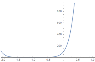
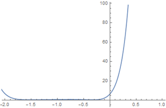
Following Liao [21, 22], the convergence of the series for HAM strongly depends on non-zero auxiliary parameters $\hbar_{f}, \hbar_{\theta}$ and $\hbar_{\emptyset}$ which helps in controlling the convergence region of the series solution. However, the admissible range values of $\hbar_{f}, \hbar_{\theta}$ and $\hbar_{\emptyset}$ are obtained by the 10th-order approximation of the HAM at M=1, $D u=0.1, \beta=1$,
$E c=0.1, S r=0.1, P r=0.72, S c=0.24, K=0.1, Q=$-0.5 at the range where $\hbar-$curve becomes parallel which gives $-1.6 \leq h_{f} \leq-0.4,-1.7 \leq \hbar_{\theta} \leq-0.2$ and $-1.2 \leq$ $\hbar_{\emptyset} \leq-0.3$ for $\hbar_{f}, \hbar_{\theta}$ and $\hbar_{\emptyset}$ respectively as shown in Figures $2-4$ below.
Figure 2. $\hbar_{f}$ -curve of $f^{\prime \prime}(0)$ at 10th order approximation
Figure 3. $\hbar_{\theta^{-}}$ curve of $\theta^{\prime}(0)$ at 10th order approximation
Figure 4. $\hbar_{f}$ -curve of $\emptyset^{\prime}(0)$ at 10th order approximation
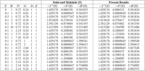
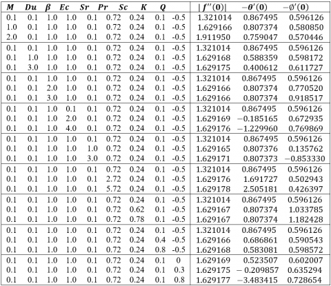
Here, we first ensure the successful implementation of the numerical result by comparing it with the previous work done. So, these present results are compared to those obtained by Seini and Makinde [5] for the local skin-friction.
Nusselt Number and Sherwood number by setting the extension over Seini and Makinde [5] results to zero, such as $Q=0, D u=0, \quad S r=0$. The results strongly agreed with each other (see Table 1).
Table 1. Comparison of the present result with Seini and Makinde [5]
In order to gain a physical understanding of the present problem, Eqns. (13)-(15) with the boundary conditions (16) and (17) have been solved using Homotopy Analysis Method (HAM) at 20th –order due to the unbounded domain, in order to meet the far-field boundary conditions. The behaviors of a various parameter such as; Magnetic Parameter (M), Radiation parameter (K), Dufour Number (Du) , Prandtl Number (Pr) Schmidt Number (Sc), Soret Number (Sr), Heat Absorption Parameter (Q), Eckert Number (Ec), and Reaction rate parameter $(\beta)$ on Velocity, Temperature, Concentration is presented graphically while the Local Skin-friction, Nusselt Number and Sherwood number were presented numerically in a tabular form.
During the computational analysis of the results, we hold $M=1, D u=0.1, S r=0.1, \beta=1, P r=0.72, S c=$ $0.24, Q=-0.5, K=0.1, E c=0.1$ constant and vary each parameter as shown in the figures below.
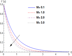
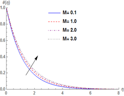
Figures 5-7 respectively presents the influence of the magnetic parameter (M) on velocity and temperature profile. It can be seen from Figure 1 that velocity distribution across the boundary layer decreases as the magnetic parameter increases. This result strongly agreed with the expectation because of the application of the magnetic field, an electrically conducting fluid that produces resistive force, called Lorentz force, which resist the motion of fluid flow within the boundary layer. The effect of Lorentz force causes frictional heating thereby results on the increase in fluid temperature and consequently boosts thermal layer thickness. It is interesting to note that the presence of (M) enhances the local skin-friction (see Table 2), which magnifies the shear stress and accelerates the flow.
Table 2. Numerical values of the skin-friction coefficient, Local Nusselt number, and Local Sherwood number
Figure 5. Velocity profiles for different M
Figure 6. Temperature profiles for different values of M
Figure 7 depicts the effect of Prandtl number (Pr) which ranges from 0.72(Air) to 7.1(Water) on the temperature profile. The temperature distribution within the boundary layer falls for larges of Pr, which in turn declines the thickness of the thermal boundary layer. This reveals that smaller values of Pr possess high thermal conductivity and cause the heat to diffuse away quickly from the surface than higher values. It is noteworthy that the presence of P r>0 enhances the Nusselt number, which in turns improves the rate of heat transfer (see Table 2).
Figure 7. Temperature profiles for different values of Pr
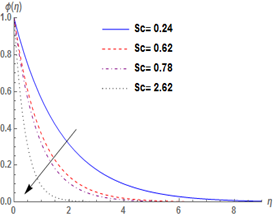
Figure 8. Concentration profiles for different values of Sc
Figure 8 illustrates the behavior of Schmidt Number (Sc) on concentration profile, which ranges from 0.24 (H2), 0.62(H2O), 0.78(NH3) and 2.62 (C9H12) (See Akinbo and Olajuwon [30]). Large values of (Sc) due to low molecular diffusivity compresses the concentration of fluid of which its aftermath declines the concentration layer thickness. Furthermore, the presence of $(S c>0)$ enhances the Sherwood number that consequently strengthens the rate of mass transfer. (see Table 2)
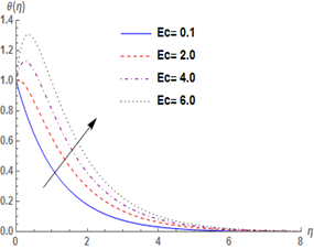
Figure 9 shows the behavior of the Eckert number (Ec) on the temperature profile. Eckert number expresses the relationship between a flow’s kinetic energy and the boundary layer enthalpy. The fluid temperature rises to its peak value within the boundary layer and suddenly falls monotonically satisfying the far-field boundary conditions. This consequently strengthens the thermal boundary layer thickness.
Figure 10 elucidates the behavior of the Radiation parameter (K) on the temperature profile. It is noticed that large values of K suggest heat from radiation processes in the operational fluid that consequently increases the temperature profile and boosts thermal layer thickness.
Figure 9. Temperature profiles for different values of Pr
Figure 10. Temperature profiles for different values of K
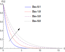
Figure 11. Temperature profiles for different values of Du
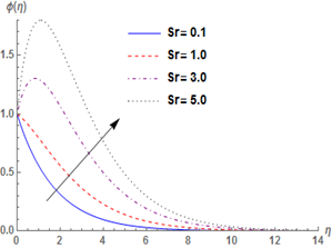
Figures 11-12 show the behaviors of Dufour and Soret numbers $(D u, S r)$ on temperature and concentration profiles. Increase in $(D u, S r)$ due to the energy flux payable to the concentration gradient and the mass flux produced by the temperature gradient demonstrate the similar increasing effect on temperature and concentration profiles respectively and thus strengthen thermal and concentration boundary layers thicknesses.
Figure 12. Concentration profiles for different values of Sr
The influence of heat absorption (Q) in temperature profile is illustrated in Figure 13. As expected, the presence of Q in the boundary layer is to absorb energy which in turn reduces the temperature of the fluid of which its aftermath reduces the thermal boundary layer thickness.
Figure 14 shows the effect of a chemical reaction $(\beta)$ on the concentration profile. Large values of R deteriorate the concentration buoyancy effect of which the resulting effect lower the concentration profile as well as its layer thickness.
Figure 13. Temperature profiles for different values of Q
Figure 14. Concentration profiles for different values of $\beta$
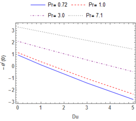
Figure 15. Effect of Du against Pr on Nusselt number $-\theta^{\prime}(0)$
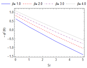
Figure 16. Effect of $S r$ against $\beta$ on Nusselt number $-\emptyset^{\prime}(0)$
The interaction between the Dufour number $(D u)$ and Prandtl number $(P r)$ is reported in Figure 15. An increase in Pr significantly improves the Nusselt number and this consequently strengthens the rate of heat transfer. However, the Nusselt number fall as the Dufour number increases against the Prandtl number which in turns lower the rate of heat transfer. A similar phenomenon is observed between Soret number $Sr$ and chemical reaction (See Figure16). It is observed that large values of $\beta$ enhance the Sherwood number which in turns boost the rate of mass transfer with a reverse phenomenon as Sr increases.
In this paper, a computational study has been carried out to analyze thermal and thermo diffusion effects on the heat and mass transfer in a viscous fluid over an exponential Stretching Surface in the presence of heat absorption. The resulting partial differential equations which describe the problem are transformed to dimensionless equations using the Similarity method with the corresponding dimensionless variables. The results of the investigation solved by the Homotopy Analysis Method (HAM) show a perfect agreement when compared with the existing literature. The effect of Lorentz force due to the magnetic interaction in the presence of heat absorption causes frictional heating thereby results in an increase in fluid temperature. A rise in heat absorption leads to a reduction of fluid temperature of which its aftermath effect results in a decrease in thermal boundary layer thickness. A similar phenomenon is also on temperature profile as large values of Pr rapidly fall the layer thickness, indicating that smaller values of Pr possess high thermal conductivity that causes the heat to diffuse away quickly from the surface than higher values.
The authors acknowledge the thoughtful comments of the anonymous referees for their useful suggestions that led to definite improvement in the paper.
|
M |
Magnetic field parameter |
|
K |
radiation parameter |
|
Pr Ec |
prandtl number Eckert number |
|
β Q Sr Du Sc |
Reaction rate parameter Heat Absorption parameter Soret Number Dufour Number Schmidt number |
|
Greek symbols |
|
|
ղ |
Similarity variable |
|
ψ |
Stream function |
[1] Sakiadis, B.C. (1961). Boundary-layer behavior on continuous solid surfaces: I. Boundary-layer equations for two-dimensional and axi-symmetric flow. American Institute of Chemical Enginers Journal, 7(1): 26–28. https://doi.org/10.1002/aic.690070108
[2] Crane, L.J. (1970). Flow past a stretching plate. Zeitschrift fu ̈r Angewandte Mathematik und Physik, 21(4): 645–655. https://doi.org/10.1007/bf01587695
[3] Carragher, P., Crane, L.J. (1982). Heat transfer on a continuous stretching sheet. Zeitschrift fu ̈r Angewandte Mathematik und Mechanik, 62(10): 564–573. https://doi.org/10.1002/zamm.19820621009
[4] Anuar, I. (2011) MHD boundary layer flow due to an exponentially stretching sheet with radiation effect. Sains Malays, 40(4): 391-395.
[5] Seini, Y.I., Makinde, O.D. (2013). MHD boundary layer flow due to exponential stretching surface with radiation and chemical. Reaction Math. Probl. Eng., 2013: 1-7. https://doi.org/10.1155/2013/163614
[6] Partha, M.K, Murthy, P.V.S.N., Rajasekhar, G.P. (2005). Effect of viscous dissipation on the mixed convection heat transfer from an exponentially stretching surface. Heat and Mass Transfer, 41(4): 360–366. Https://doi.org/10.1007/s00231-004-0552-2
[7] Sajid, M., Hayat, T. (2008). Influence of thermal radiation on the boundary layer flow due to an exponentially stretching sheet. International Communications in Heat and Mass Transfer, 35(3): 347–356. https://doi.org/10.1016/j.icheatmasstransfer.2007.08.006
[8] Noran, N.W.K., Abdul, A.S., Ahmad, S.A.A., Zaileha, M.A. (2017). Chemical reaction and radiation effects on MHD flow past an exponentially stretching sheet with heat sink. IOP Conf. Series: Journal of Physics: Conf. Series, 890: 012025. https://doi.org/10.1088/1742-6596/890/1/012025
[9] Yasir, K., Zdenek, S., Naeem, F. (2015). On the study of viscous fluid due to exponentially shrinking sheet in the presence of thermal radiation. Thermal Science, 19(1): 191-196. https://doi.org/10.2298/TSCI15S1S91K
[10] Bidin, B., Nazar, R. (2009). Numerical solution of the boundary layer flow over an exponentially stretching sheet with thermal radiation. European Journal of Scientific Research, 33(4): 710–717.
[11] Devi, R.R., Poornima, T., Reddy, N.B., Venkataramana, S. (2014). Radiation and mass transfer effects on MHD boundary layer flow due to an exponentially stretching sheet with heat source. IJEIT, 3(8): 33-39.
[12] Jat, R.N., Gopi, C. (2013). MHD flow and heat transfer over an exponentially stretching sheet with viscous dissipation and radiation effects. Applied Mathematical Sciences, 7(4): 167–180. https://doi.org/10.12988/ams.2013.13015
[13] Chen, C.H. (2010). On the analytic solution of MHD flow and heat transfer for two types of viscoelastic fluid over a stretching sheet with energy dissipation, internal heat source and thermal radiation. International Journal of Heat and Mass Transfer, 53(19): 4264–4273. https://doi.org/10.1016/j.ijheatmasstransfer.2010.05.053
[14] Nagbhooshan, J.K., Veena, P.H., Rajagopal, K., Pravin, V.K. (2012). Flow and heat transfer over an exponential stretching sheet under the effects of a temperature gradient dependent heat sink and thermal radiation. IOSR Journal of Mathematics, 2(5): 12-19.
[15] Animasaun I.L, Adebite E.A, Fagbao A.I. (2016). Casson fluid flow with a variable thermo-physical property along exponentially stretching sheet with suction and exponentially decaying internal heat generation using homotopy analysis method. Nigerian Journal of Mathematical Society, 35: 1-17. https://doi.org/org/10.1016/j.jnnms.2015.02.001
[16] Singh, A.K. (2006). Heat transfer and boundary layer flow past a stretching porous wall with temperature gradient dependent heat sink. Journal of Energy Heat and Mass Transfer, 28(2): 109-125.
[17] Mukhopadhyay, S., Bhattacharyya, K., Layek, G.C. (2014). Mass transfer over an exponentially stretching porous sheet embedded in a stratified medium. Chemical Engineering Communications, 201(2): 272–286. https://doi.org/10.1080/00986445.2013.768236
[18] Bhattacharyya, K., Layek, G.C. (2010). Chemically reactive solute distribution in MHD boundary layer flow over a permeable stretching sheet with suction or blowing. Chem. Eng. Commun., 197(12): 1527–1540. https://doi.org/10.1080/00986445.2010.485012
[19] Chauhan, D.S., Olkha, A. (2011). Slip flow and heat transfer of a second-grade fluid in a porous medium over a stretching sheet with power-law surface temperature or heat flux. Chem. Eng. Commun., 198(2): 1129–1145. https://doi.org/10.1080/00986445.2011.552034
[20] Cortell, R. (2005). Flow and heat transfer of a fluid through a porous medium over a stretching surface with internal heat generation/ absorption and suction /blowing. Fluid Dyn. Res., 37(4): 231–245. https://doi.org/10.1016/j.fluiddyn.2005.05.001
[21] Liao, S.J, (2003). Beyond perturbation: An introduction to homotopy analysis method. Boca Raton, Fla., USA: Chapman and Hall.
[22] Liao, S.J. (2003). On the analytic solution of magnetohydrodynamic flows of non-Newtonian fluids over a stretching sheet. J Fluid Mech, 488: 189–212. https://doi.org/10.1017/S0022112003004865.
[23] Hossain, M.A., Alim, M.A., Rees, D.A.S. (1999). The effect of radiation on free convection from a porous vertical plate. International Journal of Heat and Mass Transfer, 42(1): 181-191. https://doi.org/10.1016/S0017-9310(98)00097-0
[24] Ibrahim, S.M. (2014). Dissipation and variable viscosity on steady MHD free convection flow over a stretching sheet in presence of thermal radiation and chemical reaction. Advances in Applied Science Research, 5(2): 246-261.
[25] Süngü, İ.Ç. (2017). Numerical investigation on MHD flow and heat transfer over an exponentially stretching sheet with viscous dissipation and radiation effects. ITM Web of Conferences, 13: 01025. https://doi.org/10.1051/itmconf/20171301025
[26] Hussain, S.M., Sharma, R., Seth, G.S., Mishra, M.R. (2018). Thermal radiation impact on boundary layer dissipative flow of Magneto-nanofluid over an exponentially stretching sheet. International Journal of Heat and Technology, 36(4): 1163-1173. Https://doi.org/10.18280/ijht.360402
[27] Farooq, U., Zhao, Y.L., Hayat, T., Alsaed, A., Liao, S.J. (2015). Application of the HAM-based Mathematica package BVPh 2.0 on MHD Falkner-skan flow of nanofluid. Computer and Fluid, 111: 69-75. https://doi.org/10.1016/j.compfluid.2015.01.005
[28] Hayat, T., Asad, S., Mustafa, M., Hamed, H.A. (2014). Heat transfer analysis in the flow of Walters’ B fluid with a convective boundary condition. Chinese Physics B, 23(8): 084701-7. https://doi.org/10.1088/1674-1056/23/8/084701
[29] Akinbo, B.J., Olajuwon, B.I. (2019). Homotopy analysis investigation of heat and mass transfer flow past a vertical porous medium in the presence of heat source. International Journal of Heat and Technology, 37(3): 899-908. https://doi.org/10.18280/ijht.37032
[30] Akinbo, B.J., Olajuwon, B.I. (2019). Convective heat and mass transfer in electrically conducting flow past a vertical plate embedded in a porous medium in the presence of thermal radiation and thermo diffusion. Computational Thermal Sciences, 11(4): 367–385. https://doi.org/10.1615/ComputThermalScien.2019025706