Sayed Ehsan Mousavi | Saeid Kheradmand* | Mohsen Agha Seyed Mirzabozorg
© 2019 IIETA. This article is published by IIETA and is licensed under the CC BY 4.0 license (http://creativecommons.org/licenses/by/4.0/).
OPEN ACCESS
The present work is focused on numerical analysis of combustion instabilities affected by oscillating inlet flows. A non-premixed flame is considered for this purpose. First, oscillations in fuel flow was investigated. In this case different frequencies and amplitudes were investigated where instabilities were observed for the frequencies lower than 75 Hz in form of blow-off. These instabilities are also dependent on the amplitude of oscillations. As the frequency increases up to 25 Hz the amplitude of oscillations, which is the cause of flame instabilities, decreases so that in the frequency of 25 Hz the critical amplitude is 0.45 m. As the frequency surpasses 25 Hz the critical amplitude increases. The effect of oscillations in air flow on the flame behavior is also studied. In this case instability was observed as flashback where frequency is the dominant factor so that even small amplitude oscillations yield flashback. The critical frequency for oscillations in air flow is 1100 Hz so the frequencies below this limit cause instability. Also, when simultaneous oscillations of air and fuel flow were applied, both forms of flashback and blow-off were observed depending on the frequencies.
combustion instability, oscillating inlet, flashback, blow-off
Combustion instability is a consequence of complicated feedbacks from the interaction between periodic flow fields, chemical kinetics, released heat and pressure fluctuations. The resultant instabilities cause vibrations in system, increase thermal stress on walls, also lead to flame blow-off and flashback. Thus, investigation of this phenomenon is of great importance regarding its wide range of application, namely industrial gas turbines, furnaces and burners.
Although combustion instability has been studied by several researchers previously, the subject is still investigated to date due to its complicacy. Fleifil et al. [1] in 1996 proposed an analytical model to describe the dynamic response of a steady laminar premixed flame. Lieuwen and Zinn [2] in 1998, theoretically studied combustion instabilities in gas turbines with low NOx emissions in lean premixed condition. They showed that the interaction between combustion chamber pressure and the inlet velocity of reactants induce combustion instabilities. This interaction causes fluctuations in equivalence ratio which are conveyed through intake channel to combustion chamber by the main flow. This causes high-amplitude fluctuations in released heat which in turn give rise to combustion instabilities. Their results indicated that the fluctuations in equivalence ratio plays a key role in the excitement of combustion instability in gas turbines of this kind. Lee et al. [3] in 2000 proposed novel measurements of equivalence ratio fluctuations in combustion instability mode for a lean premixed flame in a particular combustion chamber. They applied infrared technic to measure equivalence ratio in the combustion chamber of a gas turbine and calibrated it for pressures and temperatures higher than 600 kPa and 683 K, respectively. Chaparro and Cetegen [4] in 2006 conducted an experiment on three types of bluff bodies. They studied flame stability in a propane premixed burner with oscillating flow at different frequencies. They concluded that the equivalence ratio at which flame separation occurs depends on the frequency of inlet flow. Fritsche et al. [5] in 2007 conducted experimental investigations to discover stable flames of both kind lean and rich. In this study a set of stable and unstable flame types were revealed based on inlet temperature and equivalence ratio.
In addition, Chaudhuri and Cetegen [6] in 2008 studied turbulent flame blow-off stabilized by bluff body with upstream spatial mixture gradients and velocity oscillations. These researchers signified a correlation between equivalence ratio and spatial mixture gradient. Zhao and Morgans [7] in 2009 implemented a passive control method in order to damp combustion instabilities. Lilleberg et al. [8] in 2009 investigated the USR model response to variations in inlet flow rate, temperature and equivalence ratio. In addition, they compared the chemical kinetics mechanism used by Lieuwen and a detailed kinetics mechanism for propane as well as methane. They proved that equivalence ratio is of great importance in combustion instability. Qiao et al. [9] in 2010 conducted experimental and numerical studies to investigate the effect of adding diluents on the extinction of an air/methane premixed flame. The extinction was traced by carbon dioxide, nitrogen and argon through thermal and radiation loss. Due to a high thermal diffusion coefficient, helium needs more energy at the onset of combustion process compared to that for other species while when using carbon dioxide as the diluent, both physical and chemical phenomena are effective. Hernández et al. Mansour et al. [10] in 2012 designed and developed a highly stabilized concentric flow conical nozzle burner for partially premixed flames. They investigated the stabilization mechanism based on two dimensional measurements of flow and temperature fields. Hernández et al. [11] in 2013 studied the concept of flame stabilizing using biomass gasification gas. They showed that the natural gas derived from biomass combustion has a higher laminar burn rate which in turn results in lower NOx emission, however it augments flashback region. Oh et al. [12] in 2013 studied the effect of adding hydrogen to a non-premixed oxy-methane flame. The experiments were carried out for different fuel jet and oxygen velocities. They found that as hydrogen mole fraction increases, flame stabilization improves.
Furthermore, Fan et al. [13] in 2013 studied the effect of blockage ratio of bluff body on hydrogen/air flame instability in a particular combustion chamber. The results indicated that there is a direct relationship between flame instability and blockage ratio of the bluff body. Also, Fan et al. [14] in 2014 numerically investigated the shape of bluff body on blow-off limit. Hydrogen and oxygen were considered as the fuel and oxidizer, respectively. The result of this study signified a higher flame stability for semicircular bluff body compared to triangular one. Also they concluded that the effect of heat loss on blow-off limit is not significant. Oh and Noh [15] in 2014 experimentally investigated the influence of CO2 diluent in a methane/air non-premixed flame. Their aim was to study the effect of adding carbon dioxide with different mole fractions to oxidizer jet on flame stability and behavior. They showed that as CO2 mole fraction increases flame stability deteriorates. Li et al. [16] in 2016 studied the angle of swirl flow in a hybrid combustor and analyzed its effect on combustion dynamics as well as NOx formation. Using LES method, these researchers attempted to find a range of swirl angles in which combustion is stable. In 2017, Khalil and Gupta [17] experimentally studied mixtures of oxygen, CO2 and methane in terms of flame stability. They particularly examined the effect of carbon dioxide dilution on flame fluctuations and realized that increasing CO2 (the diluent) to a certain extent increases the flame fluctuations while further increasing of the diluent results in a more stable flame.
In the present work, the effect of oscillating inlet flows on combustion instability is numerically studied. First, the effect of oscillations in fuel flow rate is studied. Different frequencies and amplitudes are considered for this purpose. Next, the effect of oscillations in inlet air flow is investigated. In the end, the effect of simultaneous oscillations of both fuel and air flows is studied.
The simulation is performed using Open Foam software. Perfectly Stirred Reactor (PSR) model is applied to simulate the combustion process. The model has been proved to be a feasible method for this purpose [18-20]. Also, RNG k-ε model is used to simulate the turbulence.
The following equations are applied in Favre averaged form for transient compressible flow [21]. Mass conservation equation is given as:
$\frac{\partial \bar{\rho}}{\partial t}+\frac{\partial}{\partial x_{j}}\left(\bar{\rho} \tilde{u}_{j}\right)=0$ (1)
where, $\rho$ denotes density and $u_{j}$ is the $x_{j}$ -direction velocity component. Also, the tilde shows Favre averaged terms and overbar pertains to Reynolds averaged terms. Mean momentum conservation is defined as:
$\frac{\partial}{\partial t}\left(\bar{\rho} \widetilde{u}_{\imath}\right)+\frac{\partial}{\partial x_{l}}\left(\bar{\rho} \widetilde{u}_{\imath} \widetilde{u}_{\jmath}\right)=-\frac{\partial \bar{p}}{\partial x_{j}}+\frac{\partial}{\partial x_{j}}\left(\bar{\tau}_{i j}-\bar{\rho} \widetilde{u_{\imath}^{\prime \prime} u_{\jmath}^{\prime \prime}}\right)+\bar{\rho} \widetilde{F}_{\imath}$ (2)
where, p is pressure, $\tau_{i j}$ and $F_{i}$ are viscous stress tensor and body-force acceleration in $x_{i}$ -direction, respectively. Also, transport equation in terms of mean mass fraction is:
$\begin{aligned} & \frac{\partial}{\partial t}\left(\bar{\rho} \tilde{Y}_{k}\right)+\frac{\partial}{\partial x_{j}}\left(\bar{\rho} \tilde{Y}_{k} \tilde{u}_{j}\right) =\frac{\partial}{\partial x_{j}}\left(\bar{\rho} D \frac{\partial \tilde{Y}_{k}}{\partial x_{j}}\right)-\frac{\partial}{\partial x_{j}}(\bar{\rho} \overline{u_{j}^{\prime \prime} Y_{k}^{\prime \prime}})+\overline{\omega_{k}} \\ k &=1, \ldots, N_{s p e c i e s} \end{aligned}$ (3)
where, $\tilde{Y}_{k}$ is the mean mass fraction of an individual species in a mixture of N species. Also, D is the diffusion coefficient and $\omega_{k}$ denotes species $k$ net production volumetric rate as a result of chemical reaction. Considering total enthalpy h, the energy transport equation is:
$\frac{\partial}{\partial t}(\bar{\rho} \tilde{h})+\frac{\partial}{\partial x_{j}}\left(\bar{\rho} \tilde{h} \tilde{u}_{j}\right)=\frac{\partial}{\partial x_{j}}\left(\bar{\rho} \alpha \frac{\partial \tilde{h}}{\partial x_{j}}-\bar{\rho} \widetilde{u_{j}^{\prime \prime} h^{\prime \prime}}\right)+\bar{S}$ (4)
where, $\alpha$ and S are thermal diffusivity and thermal energy produced internally, respectively. The following equation accounts for the Reynolds stresses:
$\bar{\rho} \widetilde{u_{i}^{\prime \prime} u_{j}^{\prime \prime}}=-\mu_{t}\left(\frac{\partial \tilde{u}_{i}}{\partial x_{j}}+\frac{\partial \widetilde{u}_{j}}{\partial x_{i}}-\frac{2}{3} \delta_{i j} \frac{\partial \widetilde{u}_{k}}{\partial x_{k}}\right)+\frac{2}{3} \bar{\rho} \tilde{k} \delta_{i j}$ (5)
where, $\delta_{i j}$ denotes Kronecker delta. Also, eddy viscosity $\mu_{t}$ is defined as:
$\mu_{t}=\frac{C_{\mu} \bar{\rho} \tilde{k}^{2}}{\tilde{\varepsilon}}$ (6)
where, $C_{\mu}$ is a constant, $k$ is Turbulence kinetic energy and $\varepsilon$ denotes turbulence kinetic energy dissipation rate. For the turbulence fluxes in Equations 3 and $4,$ gradient model is given as:
$-\bar{\rho} \widetilde{u_{\imath}^{\prime \prime} Y_{k}^{\prime \prime}}=\frac{\mu_{t}}{\sigma_{t}} \frac{\partial \tilde{Y}_{k}}{\partial x_{i}}$ (7)
$-\bar{\rho} \widetilde{u_{i}^{\prime \prime} h^{\prime \prime}}=\frac{\mu_{t}}{\sigma_{t}} \frac{\partial \widetilde{h}}{\partial x_{i}}$ (8)
where, $\sigma_{t}$ is a constant. Turbulence kinetic energy, k, is defined as:
$\frac{\partial}{\partial t}(\bar{\rho} \tilde{k})+\frac{\partial}{\partial x_{i}}\left(\bar{\rho} \tilde{u}_{i} \tilde{k}\right)=\frac{\partial}{\partial x_{i}}\left[\left(\mu+\frac{\mu_{t}}{\sigma_{k}}\right) \frac{\partial \tilde{k}}{\partial x_{i}}\right]+G-\bar{\rho} \tilde{\varepsilon}$ (9)
where, $\sigma_{k}$ is a constant and $G$ is the rate of turbulence kinetic energy production defined as:
$G=-\bar{\rho} \widetilde{u_{l}^{\prime \prime} u_{j}^{\prime \prime}} \frac{\partial \widetilde{u}_{i}}{\partial x_{j}}$ (10)
Also, turbulence kinetic energy dissipation rate, $\varepsilon,$ is given as:
$\frac{\partial}{\partial t}(\bar{\rho} \tilde{\varepsilon})+\frac{\partial}{\partial x_{i}}\left(\bar{\rho} \tilde{u}_{i} \tilde{\varepsilon}\right)=\frac{\partial}{\partial x_{i}}\left[\left(\mu+\frac{\mu_{t}}{\sigma_{\varepsilon}}\right) \frac{\partial \tilde{\varepsilon}}{\partial x_{i}}\right]+C_{\varepsilon 1} \frac{\tilde{\varepsilon}}{\tilde{k}} G-C_{\varepsilon 2} \bar{\rho} \frac{\tilde{\varepsilon}^{2}}{\tilde{k}}$ (11)
where, $\sigma_{\varepsilon}, C_{\varepsilon 1}$ and $C_{\varepsilon 2}$ are constants. The following values are recommended by $[21,22]$ for the model constants: $\sigma_{k}=1$ $\sigma_{t}=0.7, \sigma_{\varepsilon}=1.3, C_{\mu}=0.09, C_{\varepsilon 1}=1.44$ and $C_{\varepsilon 1}=1.92$.
In this section the possibility of combustion instability due to various factors are investigated and the regions prone to instability are determined. At first, validation of the numerical approach is presented, next the effect of oscillating inlet flow on flame behavior is included.
3.1 Validation
3.1.1 Transient condition
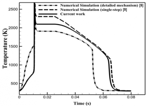
The results of the present work are compared against the numerical studies of Lilleberg et al. [8]. They performed two types of numerical simulations: first, a simulation using detailed mechanism with 325 elementary reactions. Second, a simulation using single step mechanism, whose results are compared to the results of the detailed mechanism simulation.
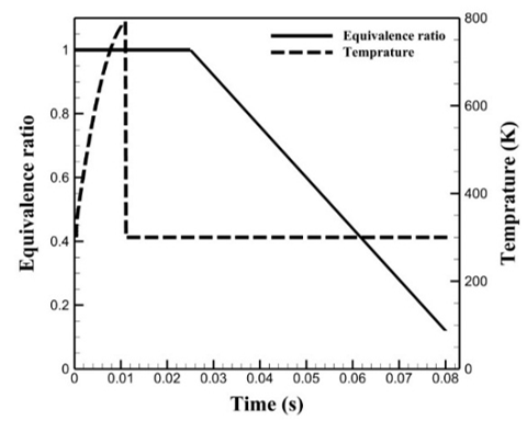
In the present study, a single step mechanism is applied and the model of a premixed reactor is considered for combustion and extinction simulations. Figure 1 depicts equivalence ratio and flow temperature at the reactor inlet. Temperature rises gradually until combustion occurs. Afterward, inlet flow temperature is decreased to 300 K. Equivalence ratio is equal 1 until 0.025 s, then decreases.
Figure 1. Equivalence ratio and inlet flow temperature as a function of time
Figure 2 depicts the reactor temperature as a function of time and compares the present work with the results presented by Lilleberg et al. [8]. The reactor temperature is equal to the inlet flow temperature until the onset of combustion after which the steady state condition is attained. Then it decreases in accordance with the decrease of equivalence ratio. As the charge gets lean, extinction occurs and the temperature falls to the inlet temperature again.
As shown in Figure 2, the maximum discrepancy for the present work is found to be 10.5 percent in comparison with the results of the numerical study with 325 reactions and 53 species. The comparison shows that the present study has done a better job compared with the single step simulation performed by the reference [8], meaning the present results are closer to the results of the simulation with detailed mechanism.
Figure 2. Validation of numerical approach for transient condition (Reactor temperature vs. time)
3.1.2 Steady state condition
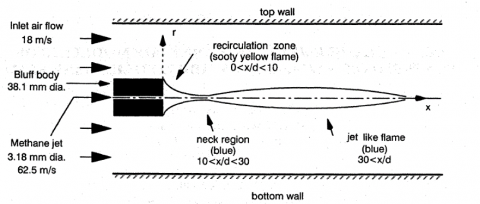
The experimental study by Correa et al. [23] about air/methane non-premixed combustion is used for validation of the present numerical approach in steady state condition. A zero dimensional model is implemented using PSR concept and the Favre-averaged equations are solved in steady state condition. Fuel and air velocities are set to 62.5 and 18 m/s, respectively, and inlet pressure is atmospheric. Figure 3 presents the geometrical characteristics.
Figure 3. Flame geometry [23]
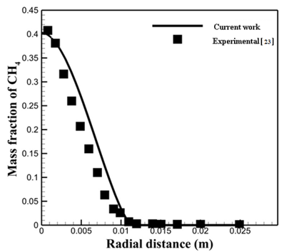
Figure 4. Validation of the numerical approach for steady state condition
Figure 4 shows methane mass fraction as a function of radial distance from the center. Mass fraction decreases as the distance from the center and from fuel inlet increases. The results of the current work are close to the experimental data, signifying the numerical approach for steady mode is reliable.
3.2 Grid dependency
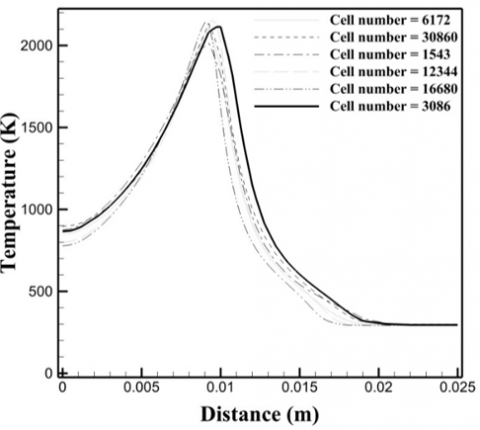
A structured mesh is applied to the computational domain. Increasing the number of grids improves the results at the expense of computational time. Therefore, a grid study is performed to achieve the optimum number of grids. Figure 5 depicts temperature variation along the radial distance of the combustor at the axial distance of 0.052 m from inlet for different grid numbers. Increasing the grid numbers larger than 3086 do not bring about a significant improvement, thus, 3086 cells are considered to minimize the computation time and cost.
Figure 5. Temperature variation along the radial distance of the combustor for different cell numbers
3.3 Combustion instability due to inlet oscillations
The flame geometry considered for this study is analogous to that depicted in Figure 3. Fuel and air are introduced to the reactor at velocities of 62.5 and 18 m/s, respectively. Also, the inlet pressure is atmospheric in all cases. At first, results for fuel oscillations, next air oscillations and in the end simultaneous oscillations in fuel and air are presented.
3.3.1 Fuel flow oscillations
In this section, oscillation is applied to fuel flow in various amplitudes and frequencies in the form of Eq. (12):
$U=U_{s t}[1+\mathrm{A} \cos (2 \pi f t)]$ (11)
where, U and Ust denote oscillating velocity and steady state velocity, respectively. Also, A is the amplitude of oscillations and f and t represent frequency and time, respectively. It takes 0.1 s for the flame to reach steady state after which it is subjected to oscillation. The study begins with the case with the frequency and amplitude of 25 Hz and 0.8 m, respectively. The study is carried out for 10 periods and the moments of blow-off occurrence is determined.
Flame blow-off occurs at 0.1065, 0.1427, 0.1828, 0.2228, 0.2628, 0.3028, 0.3428, 0.3828, 0.4228 s. Given these time steps one can realize that instability occurs periodically in this case. The fifth cycle is considered for further studies and the oscillation of fuel flow is applied with a frequency and amplitude of 25 Hz and 0.8 m, respectively. In order to achieve more details on this phenomenon, various parameters are studied at the axial distance of 0.052 m from inlet where blow-off has occurred.
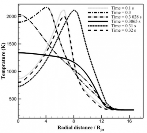
Figure 6 presents temperature as a function of a dimensionless parameter which is defined as the radial distance, r, divided by the inlet fuel jet radius, R. In the fifth period, the following time steps are studied: 0.3, 0.3028, 0.3065, 0.31, and 0.32 s with corresponding velocities of 25.5, 17.12, 36.37, 62.5, and 112.5 m/s, respectively.
The curve for the time step of 0.1 s pertains to the steady state condition. It increases to a maximum then drastically falls. In fact, temperature rises due to an increase in the fuel mass participating in reaction while the opposite occurs for the decreasing region. The temperature curve for 0.3 s starts from 1900 K and decreases for r/R larger than 4. As it is shown, in the increasing region the dimensionless distance is smaller compared with that in the decreasing region. This is due to the high unmixedness factor of 0.9 at this time step (values close to 1 signify a proper unmixedness of fuel and air). In the fifth cycle, blow-off occurs at 0.3028 s and the corresponding temperature curve starts from 2000 K and falls continuously. It can be seen in Figure 6 that extinction occurs at 0.3065 s that is slightly after the occurrence of blow-off at 0.3028 s. Also, Figure 6 depicts flame thickness, 3.2 units at 0.1 s and 4 units at the moment of blow-off. Despite the same fuel velocities at 0.1 and 0.3 s, temperature curves are different at these time steps. On the other hand the temperature curves for 0.1 and 0.32 s are the same while the fuel velocity at 0.32 s is 112.5 m/s. The reason for this lag is that it takes a while for upstream fluctuations to affect downstream. All cases tend to reach the air temperature at the maximum radial distance.
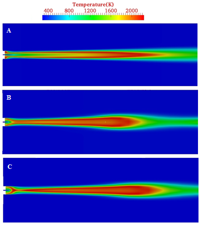
Figure 7a depicts temperature distribution in the combustion chamber at 0.1 s which corresponds to the steady state condition before the onset of oscillations. Figure 7b shows temperature distribution in combustion chamber at the lowest fuel flow velocity, 12.5 m/s and Figure 7c shows temperature contour at 0.3028 s when blow-off occurs.
Figure 6. Combustion chamber temperature combustion chamber at different time steps
Figure 7. Combustion chamber temperature contours at 0.1 s (A), 0.3 s (B), and 0.3028 s (C)
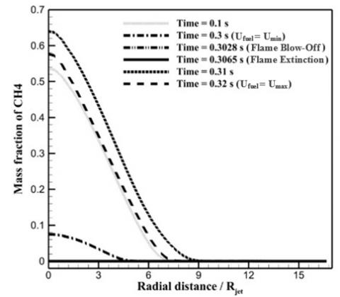
Figure 8 depicts methane mass fraction for the studied time steps. At 0.1 s the mass fraction starts at 0.54 for the dimensionless distance of zero and ends to 0 at dimensionless distance of 7. The reason is that r/R of 7 is far from the fuel inlet and rather close to the air inlet. At the moment of blow-off, i.e. 0.3028 s, and before r/R of 4.2, methane mass fraction is slightly larger than zero while after that distance it becomes zero. This is due to the fact that at this time step the entering fuel takes part in reaction and burns up, keeping methane mass fraction about zero. Also, at the moment of extinction, methane mass fraction is found to be zero all over the radial distance. In fact, all the fuel entering the combustion chamber generates a rather short flame at the inlet; therefore, no fuel mass reaches the axial distance of 0.052 m which is the location depicted in Figure 8. Also, the mass fraction remains zero at this time step along the radius of the chamber. Mass fraction curve for the time step of 0.3 s starts from 0.08 at r/R of 0 and decreases continuously. By comparing Figure 6 with Figure 8 for this time step it can be noted that up to r/R of 4.2 the amount of available fuel is more than the fuel participating in reaction. Also, for the r/R values in the range of 4.2 to 5, the flame causes the methane to burn up which in turn results in a mass fraction of zero in this radial distance.
Figure 8. Methane mass fraction at the axial distance of 0.052 m
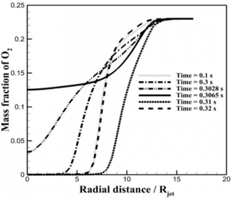
Figure 9 presents oxygen mass fraction as a function of the dimensionless distance parameter at the axial distance of 0.052 m. It pertains to inlet air velocity of 18 m/s. At this time, inlet fuel is subjected to oscillations. Oxygen mass fraction at 0.1 s is zero for r/R values of 0 to 6. For r/R values larger than 6, oxygen mass fraction drastically rises up to 0.23. The zero mass fraction of oxygen for r/R between 0 and 0.4 is explained by the fact that no air is present at this time (as shown in Figure 12 for nitrogen mass fraction). For r/R values of 0.4 to 6, oxygen completely takes part in reaction and burns up. In the end, the mass fraction reaches up to 0.23 because the corresponding radial distance is far away from the fuel inlet so that no reaction occurs at that location, therefore the air remains unused. At the moment of blow-off, oxygen mass fraction starts from 0.023 and ends to 0.23. Oxygen mass fraction has a nonzero value at all radial locations which is due to the fact that the present oxygen is not properly mixed with methane and a large amount of it does not participate in reaction. At the time step corresponding to extinction, mass fraction starts at 0.125 and ends to 0.23 and for the time step of 0.31 s it remains zero up to r/R of 7.5, then starts to increase. In fact, air is not present up to r/R of 2 and from that on oxygen starts to participate in reaction.
Figure 9. Oxygen mass fraction at the axial location of 0.052 m
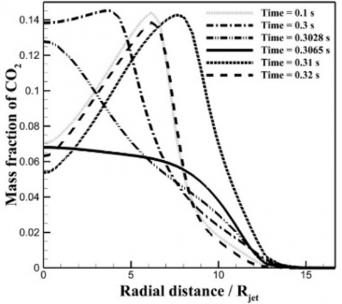
Figure 10 depicts carbon dioxide mass fraction at the axial distance of 0.052 m as a function of r/R. For the time step of 0.1 s, when the inlet fuel is not subjected to oscillations yet, mass fraction starts from 0.07 and rises to its maximum, 0.14, at r/R of 6. After that, it falls to zero at r/R of 12.5. The increasing region is due to the ongoing burning reaction and subsequent decrease in mass fraction of methane (Figure 8), also it is due to the fact that the reaction itself generates carbon dioxide. On the other hand the decreasing region is due to lack of combustion reaction at the axial distances larger than 7.4 (Figure 6). At 0.3 s, mass fraction starts from 0.14 and increases to its maximum then diminishes. It should be pointed out that at 0.3 s fuel flow rate is minimum. For r/R of 0 to 5, the oxygen totally burns up in reaction which generates carbon dioxide and results in a rise in its mass fraction. After r/R of 5 it falls due to the decrease in combustion reaction and increase in oxygen mass fraction. At the moment of blow-off, carbon dioxide mass fraction starts from 0.125 and diminishes continuously.
Also, for the time steps of 0.31 and 0.32 s, carbon dioxide mass fraction variations are similar such that they increase to their maximum then decrease to 0. The reason for this behavior is that despite the abundancy of fuel near the center line (small r/R values) the amount of oxygen is not significant, not adequate for the fuel to burn up completely. As r/R increases, the amount of oxygen rises, resulting in a more proper mixing. This trend continues until the best mixing is provided, generating more carbon dioxide. After the peak, the amount of oxygen rises progressively while the fuel mass decreases to zero in the end. Therefore, no combustion occurs and carbon dioxide mass fraction becomes zero.
In addition, Figure 10 indicates that at the moment of blow-off carbon dioxide mass fraction at the center line (r/R equal 0) is less than that for the time step of 0.3 s. However, in Figure 6 this is converse for temperature, simply because more mass requires more heat to reach the combustion temperature. This fact leads to a drop in temperature.
Figure 10. Carbon dioxide mass fraction at the axial distance of 0.052 m
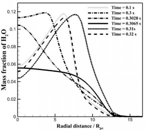
Figure 11 depicts H2O mass fraction as a function of r/R. At the time step of 0.1 s, meaning steady state condition, H2O mass fraction starts from 0.058 at the center line (r/R=0) and reaches the maximum at r/R of 6, while from this point on it diminishes continuously. In fact, before the maximum, H2O is generated as a product of the ongoing combustion reaction, thus mass fraction is increasing. Afterward, the combustion reaction is over and mass fraction of H2O decreases. Also, as it can be noted in Figure 11 at 0.3 s mass fraction curve has two distinct parts. In the first part, before r/R of 5, mass fraction is slowly increasing while at the next region, after r/R of 5, it rises rapidly. The reason is that in the first region the presence of both oxygen and methane leads to combustion while in the next region the reaction gradually stops due to the lack of proper mixing, therefore methane mass fraction falls to zero (Figure 8). Also, as it is depicted in Figure 6, flame does not exist after r/R of 6. At the moment of flame blow-off, mass fraction starts at its maximum value at r/R of 0 and diminishes to 0 continuously. The reason for this trend is that as the radial distance increases, burning reaction mitigates that diminishes the amount of combustion products.
Figure 11. H2O mass fraction at the axial distance of 0.052 m
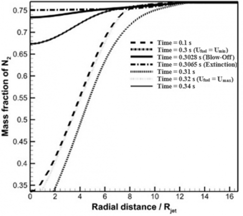
Figure 12 presents nitrogen mass fraction as a function of r/R at different time steps. For the time step of 0.1 s the mass fraction remains zero up to r/R of 0.8 while after this r/R it increases rapidly up to 0.77. Given the fact that nitrogen does not participates in the reaction, no air is present where nitrogen mass fraction is zero. On the other hand, a mass fraction equal to 0.77 means that only air is present. At the time step of 0.3, when oscillations are applied, mass fraction starts at 0.75 and ends to 0.77. At this time step, which corresponds to the minimum fuel flow rate, air is able to reach all over the chamber. This results in a nonzero mass fraction of nitrogen for all r/R values.
Figure 12. Nitrogen mass fraction at the axial distance of 0.052 m
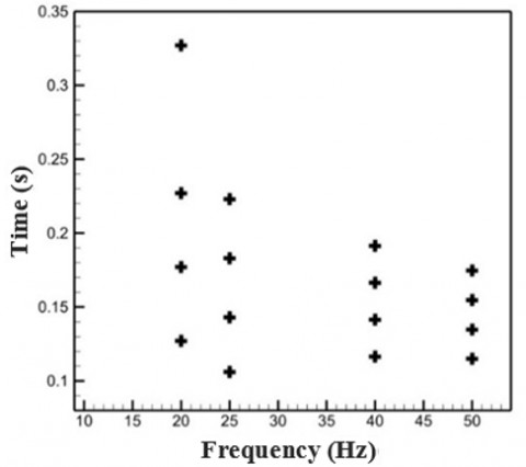
Frequency of Fluctuations in Instability Mode. Figure 13 depicts the time at which blow-off occurs versus the frequency of fuel flow oscillations. The period of oscillation is determined as the time gap between two blow-off occurrences for a given frequency.
Figure 13. Effect of frequency on instability occurrence
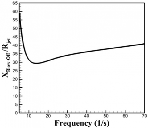
Axial Distance of Blow-Off Location. Figure 14 depicts the location of flame blow-off versus frequency. The blow-off location is presented as the radial distance at which it occurs divided by the fuel jet radius. Flame blow-off starts from r/R of 59 at the frequency of 5 Hz and diminishes to its minimum value then slowly rises. Low frequencies are close to steady condition (no oscillation) indicating the time step of 0.1.
Figure 14. Effect of frequency on the location of blow-off
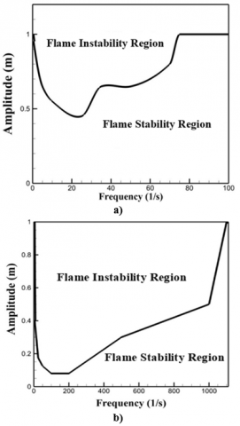
Instability Region. Both stable and unstable regions are depicted in Figure 15a as a function of frequency and amplitude of oscillations in fuel flow. In fact, the flame behavior is simulated with the same air velocity but the fuel flow velocity is subjected to oscillations in different frequencies. By analyzing the results the stable regions are identified. As it is depicted in Figure 15a, at frequencies higher than 75 Hz no instability occurs which is due to the fact that it takes a certain time for upstream to impact downstream. In other words, if the period of oscillations is less than 0.01333 s blow-off does not occur.
3.3.2 Air flow oscillations
In this section, the influence of inlet air oscillations on flame behavior is investigated. In this case, combustion instability is observed as flashback. The equation applied for the oscillations is the same for fuel oscillations. Flame behavior is studied with frequency and amplitude of 25 Hz and 0.8 m, respectively, also the fuel flow velocity is maintained constant at 62.5 m/s and the steady is set to 18 m/s.
Instability Region. In Figure 15b, which depicts air velocity oscillations versus frequency, stability region is determined. At frequencies higher than 1100 Hz no flame instability is observed. Therefore, if the oscillation period is less than 9.09e-4 s, flashback does not occur.
Figure 15. Stability region for: a) oscillating fuel flow; b) oscillating air flow
3.3.3 Simultaneous oscillations in fuel and air flow
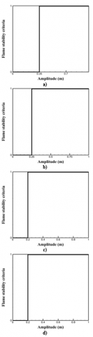
The study of simultaneous oscillations falls in two parts. The first part pertains to equal frequencies that is studied for the frequencies of 25, 50, 75 and 100 Hz. The second part focuses on unequal simultaneous frequencies. The results are presented in terms of stability criterion (0 indicates stable a flame and 1 indicates an unstable flame) as a function of amplitude.
Figure 16a depicts stable region for the frequency of 25 Hz. As it is presented, for the amplitudes smaller than 0.35 m flame is stable while for larger amplitudes instability occurs as flashback. Also, Figure 16b depicts the stable region for the frequencies of 50 and 75 Hz. In this case, unstable region starts from the amplitude of 0.25 m where flashback occurs. Stable region for the frequency of 100 Hz is presented in Figure 16c where instability appears as flashback for the amplitudes larger than 0.2 m. Also, Figure 16d shows stability criteria for the case with unequal simultaneous frequencies.
Figure 16. Stable regions for different conditions: a) equal simultaneous frequencies of 25 Hz; b) equal simultaneous frequencies of 50 and 75 Hz; c) equal simultaneous frequency of 100 Hz; d) unequal simultaneous frequencies
The results of the simulation of flame behavior with oscillating inlet flows were presented. Non-premixed flames respond to oscillating inlets in two forms, stable and unstable. Combustion instability, in this case, is observed as blow-off and flashback.
For oscillating fuel flow, the frequencies lower than 75 Hz lead to combustion instability which is observed as flame blow-off. If the frequency is higher than the limit (75 Hz) the flame remains stable. Also, at the frequencies lower than 15 Hz flame blow-off occurs near the fuel inlet while at higher frequencies it moves away from the fuel inlet.
Periodic oscillations in inlet flows directly affect flame behavior, in other words if the frequency and amplitude are in the risk region the time interval between two consecutive blow-off occurrences equals the period of oscillation.
Oscillations in fuel flow only in certain amplitudes may lead to combustion instability. Based on the results, as the frequency increases up to 25 Hz the amplitude of oscillations, which causes instabilities, decrease so that at the frequency of 25 Hz the critical amplitude is 0.45 m. Further increasing the frequency causes the critical amplitude to increase. The critical frequency for fuel oscillations was found to be 75 Hz.
Oscillations in air flow leads to two different flame behaviors: risk and risk free regions. In the risk region, the instability is observed as flashback. According to the results, the risk region is wider for air flow oscillations compared with that for fuel oscillations.
In the case of oscillating air flow, frequency is dominant over amplitude so that even small amplitudes may lead to flashback. The critical frequency in this case is 1100 Hz, meaning lower frequencies lead to instability.
When both fuel and air flows are oscillating simultaneously, if their frequency is equal, instability appears in form of flashback while for unequal frequencies instability may occur in both flashback and blow-off forms.
|
A |
amplitude |
|
a |
thermal diffusivity |
|
D |
diffusion coefficient |
|
F |
body-force acceleration |
|
f |
frequency |
|
G |
turbulence kinetic energy production rate |
|
h |
total enthalpy |
|
N |
number of species |
|
p |
pressure |
|
S |
thermal energy produced internally |
|
T |
temperature |
|
T |
time |
|
u |
velocity |
|
V |
volume |
|
Y |
mass fraction |
|
Greek ymbols |
|
|
$\varepsilon$ |
turbulence kinetic energy dissipation |
|
$\delta$ |
Kronecker delta |
|
$\rho$ |
density |
|
k |
turbulence kinetic energy |
|
$\mu$ |
viscosity |
|
$\tau$ |
viscose stress tensor |
|
$\omega$ |
net production volumetric rate |
|
Subscripts |
|
|
k |
species number |
|
t |
turbulent |
[1] Fleifil, M., Annaswamy, A.M., Ghoneim, Z., Ghoniem, A.F. (1996). Response of a laminar premixed flame to flow oscillations: A kinematic model and thermoacoustic instability results. Combustion and Flame, 106(4): 487-510. http://dx.doi.org/10.1016/0010-2180(96)00049-1
[2] Lieuwen, T., Zinn, B.T. (1998). The role of equivalence ratio oscillations in driving combustion instabilities in low NOx gas turbines. Proc. Symposium (International) on combustion, Elsevier, pp. 1809-1816. http://dx.doi.org/10.1016/S0082-0784(98)80022-2
[3] Lee, J.G., Kim, K., Santavicca, D. (2000). Measurement of equivalence ratio fluctuation and its effect on heat release during unstable combustion. Proceedings of the Combustion Institute, 28(1): 415-421. http://dx.doi.org/10.1016/S0082-0784(00)80238-6
[4] Chaparro, A.A., Cetegen, B.M. (2006). Blowoff characteristics of bluff-body stabilized conical premixed flames under upstream velocity modulation. Combustion and Flame, 144(1-2): 318-335. http://dx.doi.org/10.1016/j.combustflame.2005.08.024
[5] Fritsche, D., Füri, M., Boulouchos, K. (2007). An experimental investigation of thermoacoustic instabilities in a premixed swirl-stabilized flame. Combustion and Flame, 151(1-2): 29-36. http://dx.doi.org/10.1016/j.combustflame.2007.05.012
[6] Chaudhuri, S., Cetegen, B.M. (2008). Blowoff characteristics of bluff-body stabilized conical premixed flames with upstream spatial mixture gradients and velocity oscillations. Combustion and Flame, 153(4): 616-633. http://dx.doi.org/10.1016/j.combustflame.2007.12.008
[7] Zhao, D., Morgans, A.S. (2009). Tuned passive control of combustion instabilities using multiple Helmholtz resonators. Journal of Sound and Vibration, 320(4-5): 744-757. http://dx.doi.org/10.1016/j.jsv.2008.09.006
[8] Lilleberg, B., Ertesvåg, I.S., Rian, K.E. (2009). Modeling instabilities in lean premixed turbulent combustors using detailed chemical kinetics. Combustion Science and Technology, 181(9): 1107-1122. http://dx.doi.org/10.1080/00102200902973174
[9] Qiao, L., Gan, Y., Nishiie, T., Dahm, W., Oran, E. (2010). Extinction of premixed methane/air flames in microgravity by diluents: Effects of radiation and Lewis number. Combustion and Flame, 157(8): 1446-1455. http://dx.doi.org/10.1016/j.combustflame.2010.04.004
[10] Mansour, M.S., Elbaz, A., Samy, M. (2012). The stabilization mechanism of highly stabilized partially premixed flames in a concentric flow conical nozzle burner. Experimental Thermal and Fluid Science, 43: 55-62. http://dx.doi.org/10.1016/j.expthermflusci.2012.03.017
[11] Hernández, J.J., Lapuerta, M., Barba, J. (2013). Flame stability and OH and CH radical emissions from mixtures of natural gas with biomass gasification gas. Applied Thermal Engineering, 55(1-2): 133-139. http://dx.doi.org/10.1016/j.applthermaleng.2013.03.015
[12] Oh, J., Noh, D., Ko, C. (2013). The effect of hydrogen addition on the flame behavior of a non-premixed oxy-methane jet in a lab-scale furnace. Energy, 62: 362-369. http://dx.doi.org/10.1016/j.energy.2013.09.049
[13] Fan, A., Wan, J., Liu, Y., Pi, B., Yao, H., Maruta, K., Liu, W. (2013). The effect of the blockage ratio on the blow-off limit of a hydrogen/air flame in a planar micro-combustor with a bluff body. International Journal of Hydrogen Energy, 38(26): 11438-11445. http://dx.doi.org/10.1016/j.ijhydene.2013.06.100
[14] Fan, A., Wan, J., Liu, Y., Pi, B., Yao, H., Liu, W. (2014). Effect of bluff body shape on the blow-off limit of hydrogen/air flame in a planar micro-combustor. Applied Thermal Engineering, 62(1): 13-19. http://dx.doi.org/10.1016/j.applthermaleng.2013.09.010
[15] Oh, J., Noh, D. (2014). The effect of CO2 addition on the flame behavior of a non-premixed oxy-methane jet in a lab-scale furnace. Fuel, 117: 79-86. http://dx.doi.org/10.1016/j.fuel.2013.08.065
[16] Li, S., Fu, Z.G., Shen, Y.Z., Wang, R.X., Zhang, H. (2016). LES of swirl angle on combustion dynamic and NOx formation in a hybrid industrial combustor. International Journal of Heat and Technology, 34(2) 197-206. https://doi.org/10.18280/ijht.340207
[17] Khalil, A.E., Gupta, A.K. (2017). Flame fluctuations in Oxy-CO2-methane mixtures in swirl assisted distributed combustion. Applied Energy, 204: 303-317. https://doi.org/10.1016/j.apenergy.2017.07.037
[18] D’ERRICO, G., Lucchini, T., Montenegro, G., Zanardi, M. (2019). Development of OpenFOAM application for internal combustion engine simulation. Proc. OpenFOAM International Conference, pp. 1-25.
[19] Kong, S.C., Sun, Y., Rietz, R.D. (2007). Modeling diesel spray flame liftoff, sooting tendency, and NOx emissions using detailed chemistry with phenomenological soot model. Journal of Engineering for Gas Turbines and Power, 129(1): 245-251. https://doi.org/10.1115/1.2181596
[20] Singh, S., Reitz, R.D., Wickman, D., Stanton, D., Tan, Z. (2007). Development of a hybrid, auto-ignition/flame-propagation model and validation against engine experiments and flame liftoff. SAE Technical Paper. http://dx.doi.org/10.4271/2007-01-0171
[21] Launder, B.E., Spalding, D.B. (1983). The numerical computation of turbulent flows. Numerical Prediction of Flow, Heat Transfer, Turbulence and Combustion. Elsevier, 96-116. http://dx.doi.org/10.1016/B978-0-08-030937-8.50016-7
[22] Jones, W., Whitelaw, J. (1982). Calculation methods for reacting turbulent flows: A review. Combustion and Flame, 48: 1-26. http://dx.doi.org/10.1016/0010-2180(82)90112-2
[23] Correa, S.M., Gulati, A., Pope, S.B. (1994). Raman measurements and joint PDF modeling of a nonpremixed bluff-body-stabilized methane flame. Proc. Symposium (International) on Combustion, 25(1): 1167-1173. http://dx.doi.org/10.1016/S0082-0784(06)80755-1