Yan Shi* | Xianchuang Huang | Guanhong Feng
© 2019 IIETA. This article is published by IIETA and is licensed under the CC BY 4.0 license (http://creativecommons.org/licenses/by/4.0/).
OPEN ACCESS
The existing simulation software for geochemical reactions involving carbon dioxide (CO2) mostly focus on the reservoir, failing to take account of the wellbore. Considering the importance of temperature in geochemical reactions, this paper develops a wellbore-reservoir coupling geochemical simulation software for non-isothermal multiphase fluid. Based on TOUGHREACT v2.0, the software was programmed in Fortran in the light of the integrated wellbore-reservoir simulator T2Well, the conservation of momentum equation for one-dimensional (1D) fluid, and the drift-flux model. Targeting a CO2 plume geothermal (CPG) project in the Songliao Basin, the author compared the wellbore-reservoir coupling model and the simple reservoir model in terms of water and heat transfer, mineral dissolution and precipitation, change in pore permeability, etc. The comparison shows that CO2 in the wellbore varies greatly in temperature and pressure; the injection well is much hotter at the bottom than at the wellhead. In the region near the injection well, the two models differed slightly despite the huge temperature difference; In the region near the production well, the wellbore-reservoir coupling model predicted slightly more violent dissolution and precipitation reactions and a greater CCS amount than the other model. The research findings lay the basis for the simulation of CO2 geological engineering.
Wellbore-reservoir coupling simulation, geochemical reaction, carbon dioxide (CO2), drift-flux model
Carbon dioxide (CO2) capture and storage (CCS) is a technology aimed at reducing greenhouse gas (GHG) emissions [1]. To reduce the CCS cost, the CO2 capture, utilization and storage (CCUS) techniques were developed to utilize the CO2 before the CCS [2-4], namely, CO2-enhanced geothermal system (CO2-EGS), CO2-enhanced coal bed methane (CO2-ECBM) recovery, CO2-enhanced water recovery (CO2-EWR) and CO2-enhanced oil recovery (CO2-EOR).
The CO2-EGS was proposed by Brown in 2000 [5]. Atrens et al. predicted that the CO2-EGS would be less effective at energy extraction than a water-EGS for conditions used in past EGS trials [6]. One year later, Randolph and Saar shifted the focus from fractured medium to porous medium, and put forward the CO2 plume geothermal (CPG) technology, which uses CO2 to recover geothermal energy from sedimentary basins [7]. For CPG, many scholars studied its heat extracting efficiency, such as Luo et al. [8] and Xu et al. [9]. There are also some studies on the non- isothermal flow in CO2 sequestration engineering such as Ruan et al. [10] and Singh et al. [11], their research focus wellbore and reservoir respectively. However, no studies mentioned above considered the reactive transport process and geochemical reaction.
During the CPG operation, the CO2 injection causes the surrounding rocks to dissolve or precipitate. As a result, the geothermal reservoir will face changes in porosity, permeability and mineral composition, and thus variation in its original flow field. Then, the reservoir and the original formation water will form a water-rock-gas system, kicking off a series of complex geochemical reactions. The minerals will dissolve and precipitation in the reactions, changing the physical properties (e.g. porosity and permeability of the reservoir) [12-13].
Temperature is the key to geothermal reactions. It directly bears on the fluidity of the fluid and the geochemical reaction rate of minerals. In geochemical simulations, the temperature of the injected CO2 fluid is generally handled in two approaches. Some software assume that the injected CO2 fluid and the reservoir have the same temperature, ignoring the thermal change of reactions [14]. Some treat the temperature of the CO2 fluid on the surface as the that entering the reservoir, taking account of the thermal change of reactions [15]. However, neither of the two simulation approaches can accurately describe the temperature of the CO2 fluid entering the reservoir.
Most of the existing geochemical simulation software only focus on the reservoir, failing to consider the wellbore. In actual physical process, the wellbore, as the passage between the surface and the underground, is indispensable for all geological engineering operations. After being injected at the wellhead, the low-temperature CO2 continuously picks up heat as it flows down along the wellbore, due to the heat transfer from the surrounding rocks and the conversion of gravitational potential energy [16]. The amount of temperature rise cannot be measured without calculation. Hence, the neglection of wellbore is bound to bring prediction errors. Considering the impacts of the wellbore on geochemical reactions, the wellbore and the reservoir should be treated as a whole in geochemical simulation models.
This paper develops a wellbore-reservoir coupling geochemical simulation software for non-isothermal multiphase fluid that can accurately predict the geochemical reactions in geological engineering. Based on TOUGHREACT v2.0 [17], the software was programmed in Fortran in the light of the integrated wellbore-reservoir simulator T2Well-ECO2N [18], the conservation of momentum equation for one-dimensional (1D) fluid, and the drift-flux model [19]. Pan et al. has studied the mixture flow of CO2 and water along wellbore [20-21]. ECO2N is an EoS module developed for CO2 disposal in saline aquifer. It can deal with the phase balance of CO2 and water [22].
This paper attempts to develop a wellbore-reservoir coupling geochemical simulation software for non-isothermal multiphase multi-component fluid that can accurately simulate the geothermal reactions in the presence of CO2 and effectively solve geological and environmental problems involving one or more of the following fields: hydraulic field (H), temperature field (T) and chemical field (C).
Based on the architecture of TOUGHREACT v2.0, the wellbore-reservoir coupling module was developed. The wellbore and the reservoir were treated as two separate subareas, and their multiphase flows were illustrated with different control equations. For the wellbore, the control equation is the Darcy’s law for multiphase flow. For the reservoir, the control equation is the conservation of momentum equation for 1D fluid.
Since the conservation of momentum for multiphase flow is difficult to solve, the mixing velocity of the multiphase fluid was selected as the main variable for iteration. The drift-flux model was employed to process the mixing velocity, the drift velocity and the velocity of each phase. A unified Jacobian matrix was established for the two subareas and solved to couple the different fields. The H and T were fully coupled, while the C was partially coupled. The control equations are listed in the following table.
Table 1. The control equations of the simulation program
|
Description |
Equation |
|
|
Conservation equation for mass and energy |
$\frac{d}{dt}\int_{\mathop{V}_{n}}{\mathop{M}^{\kappa }}d\mathop{V}_{n}=\int_{\mathop{\Gamma }_{n}}{\mathop{F}^{\kappa }}\bullet nd\mathop{\Gamma }_{n}+\int_{\mathop{V}_{n}}{\mathop{q}^{\kappa }}d\mathop{V}_{n}$ |
|
|
Mass accumulation |
${{M}^{\kappa }}=\phi \sum\limits_{\beta }{{{S}_{\beta }}{{\rho }_{\beta }}X_{\beta }^{\kappa }}$ |
|
|
Mass flow |
${{F}^{\kappa }}=\sum\limits_{\beta }{X_{\beta }^{\kappa }{{\rho }_{\beta }}{{u}_{\beta }}}$ |
|
|
In reservoir |
Energy flow |
${{F}^{\kappa }}=-\lambda \nabla T+\sum\limits_{\beta }{{{h}_{\beta }}{{\rho }_{\beta }}{{S}_{\beta }}{{u}_{\beta }}}$ |
|
Energy accumulation |
${{M}^{\kappa }}=(1-\varphi ){{\rho }_{R}}{{C}_{R}}T+\varphi \sum\limits_{\beta }{{{\rho }_{\beta }}{{S}_{\beta }}{{U}_{\beta }}}$ |
|
|
Flow rate |
${{u}_{\beta }}=-k\frac{{{k}_{r\beta }}}{{{\mu }_{\beta }}}(\nabla {{P}_{\beta }}-{{\rho }_{\beta }}g) $ |
|
|
In wellbore |
Energy flow |
${{F}^{\kappa }}=-\lambda \frac{\partial T}{\partial z}-\frac{1}{A}\sum\limits_{\beta }{\frac{\partial }{\partial z}\left[ A{{\rho }_{\beta }}{{S}_{\beta }}{{u}_{\beta }}({{h}_{\beta }}+\frac{u_{\beta }^{2}}{2}+gz\cos \theta ) \right]}-q'$ |
|
Energy accumulation |
${{M}^{\kappa }}=\sum\limits_{\beta }{{{\rho }_{\beta }}{{S}_{\beta }}({{U}_{\beta }}+\frac{u_{\beta }^{2}}{2}+gz\cos \theta )} $ |
|
|
Flow rate |
${{u}_{G}}={{C}_{0}}\frac{{{\rho }_{m}}}{\rho _{m}^{*}}{{u}_{m}}+\frac{{{\rho }_{l}}}{\rho _{m}^{*}}{{u}_{d}}$ ${{u}_{L}}=\frac{(1-{{S}_{G}}{{C}_{0}}){{\rho }_{m}}}{(1-{{S}_{G}})\rho _{m}^{*}}{{u}_{m}}-\frac{{{S}_{G}}{{\rho }_{G}}}{(1-{{S}_{G}})\rho _{m}^{*}}{{u}_{d}}$ |
|
The developed program was applied to the geochemical simulation of deep plume geothermal energy. The simulation results were compared with those of TOUGHREACT v2.0, aiming to verify whether wellbore-reservoir coupling simulation is necessary and superior to simple reservoir simulation. The parameters of our model were extracted from Xu’s research [12]. The research data were measured from the Songliao Basin, northeastern China. CO2 was used to recovery deep geothermal energy and subjected to the CCS.
3.1 Conceptual model
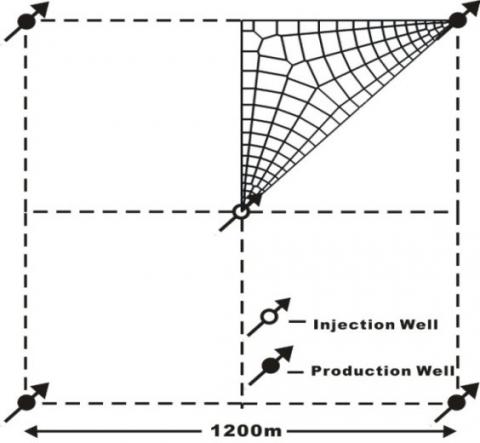
Our simulation uses a three-dimensional 3D five-point model. As shown in Figure 1, the simulation site is 1,200 m wide, and the reservoir is 50m in thickness. Considering its
Figure 1. Sketch map of the five-point model (upper right: the 1/8 simulated area)
symmetry, only 1/8 of the entire site was simulated. The simulated area was meshed nonuniformly. The meshed grids are denser in the near-well region.
The physical parameters of the reservoir were mostly cited from Xu’s research (2014) (Table 2). In the wellbore-reservoir coupling model, the wellbore diameter was set to 0.2m. The specific parameters are given in Table 2. The heat transfer between the wellbore and the surrounding rocks was interpreted by a semi-analytical solution.
Table 2. Conceptual model and physical parameters
|
Parameters of reservoir |
|
|
Depth Thickness Porosity Permeability Rock density Specific heat Heat conductivity Area of whole domain Well distance |
3800 m 5 m 0.1 1.0×10⁻¹³ m2 2650 kg/m3 920 J/kg/°C 2.51 W/m/°C 1.44 km2 848.5 m |
|
Parameters of wellbore |
|
|
Diameter Friction coefficients Specific heat Heat conductivity |
0.2 m 2.4×10⁻⁵ m 1000 J/kg/°C 2.51 W/m/°C |
3.2 Initial and boundary conditions
The reservoir was initially saturated with formation water. The initial temperature and pressure of the reservoir were 150℃ and hydrostatic pressure, respectively. For the wellhead, the initial pressure was atmospheric pressure.
For the boundary conditions, the CO2 fluid was injected at a constant flow (8kg/s), such that the wellbore-reservoir coupling model and the simple reservoir model were supplied with the same amount of CO2. To control the pressure variation in the reservoir, the recovery flow rate was set to 9kg/s in the first three years, slightly higher than the injection flow rate, and then lowered to the injection flow rate. Otherwise, if the two flow rates were the same from the very start, the reservoir will witness sharp pressure rise in the short term, for the five-point model is surrounded by zero-flow boundaries and the CO2 is much less dense than water. The operation period of the water-rock-gas system was set to 30 years. The initial and boundary conditions are detailed in Table 3.
Table 3. The initial and boundary conditions of our model
|
Initial condition |
|
|
Well bottom temperature Well bottom pressure |
150°C 36.7 MPa |
|
Boundary condition |
|
|
Injection temperature Injection mass rate Production mass rate |
20°C 8 kg/s 9 kg/s(1-3 yr)/8 kg/s(4-30 yr) |
Both relative permeability and capillary pressure play a role in the gas-liquid two-phase displacement of the model. The two factors were simulated by the van Genuchten model for relative permeability and capillary pressure. The specific parameters of the model are shown in Table 4.
Table 4. The parameters of the van Genuchten model
|
Relative permeability model |
|
|
Irreducible water saturation Irreducible gas saturation Maximum water saturation mVG |
0.15 0.01 1.00 0.65 |
|
Capillary pressure model |
|
|
Irreducible water saturation Maximum water saturation mVG Alpha Maximum capillary pressure |
0.03 1.00 0.4118 6.08×10⁻⁵Pa-1 6.4×10⁷Pa |
The mineral composition and relevant reaction kinetic parameters of the reservoir are provided in Table 5.
Table 5. Reaction kinetic parameters of primary and secondary minerals
|
Mineral |
Volume fraction |
A (cm2/g) |
Parameters for kinetic rate law |
|||||||
|
Neutral mechanism |
Acid mechanism |
Base mechanism |
||||||||
|
k25(mol/m2/s) |
Ea(kJ/mol) |
k25(mol/m2/s) |
Ea |
n(H+) |
k25(mol/m2/s) |
Ea |
n(H+) |
|||
|
Primary minerals |
||||||||||
|
Quartz |
39.0 |
9.8 |
1.02×10⁻¹⁴ |
87.7 |
||||||
|
K-feldspar |
16.0 |
9.8 |
3.89×10⁻¹³ |
38 |
8.71×10⁻¹¹ |
51.7 |
0.5 |
6.31×10⁻²² |
94.1 |
-0.823 |
|
Albite |
9.5 |
9.8 |
2.75×10⁻¹³ |
69.8 |
6.92×10⁻¹¹ |
65.0 |
0.457 |
2.51×10⁻¹⁶ |
71.0 |
-0.572 |
|
Anorthite |
5.0 |
9.8 |
7.59×10⁻¹³ |
17.8 |
3.16×10⁻⁴ |
16.6 |
1.411 |
|||
|
Kaolinite |
3.0 |
151.6 |
6.92×10⁻¹⁴ |
22.2 |
4.90×10⁻¹² |
65.9 |
0.777 |
8.91×10⁻¹⁸ |
17.9 |
-0.472 |
|
Illite |
2.0 |
151.6 |
1.66×10⁻¹³ |
35.0 |
1.05×10⁻¹¹ |
23.6 |
0.34 |
3.02×10⁻¹⁷ |
58.9 |
-0.4 |
|
Na-smectite |
2.0 |
151.6 |
1.66×10⁻¹³ |
35.0 |
1.05×10⁻¹¹ |
23.6 |
0.34 |
3.02×10⁻¹⁷ |
58.9 |
-0.4 |
|
Ca-smectite |
2.0 |
151.6 |
1.66×10⁻¹³ |
35.0 |
1.05×10⁻¹¹ |
23.6 |
0.34 |
3.02×10⁻¹⁷ |
58.9 |
-0.4 |
|
Chlorite |
2.0 |
9.8 |
3.02×10⁻¹³ |
88.0 |
7.76×10⁻¹² |
88.0 |
0.50 |
|||
|
Annite |
3.0 |
9.8 |
2.82×10⁻¹³ |
22.0 |
1.45×10⁻¹⁰ |
22.0 |
0.525 |
|||
|
Phlogopite |
3.0 |
9.8 |
2.82×10⁻¹³ |
22.0 |
1.45×10⁻¹⁰ |
22.0 |
0.525 |
|||
|
Calcite |
4.5 |
9.8 |
1.55×10⁻⁹ |
23.5 |
1.55×10⁻⁶ |
14.4 |
1.0 |
|||
|
Dolomite |
9.8 |
2.95×10⁻⁸ |
52.2 |
6.46×10⁻⁴ |
36.1 |
0.5 |
||||
|
Non-reactive |
9.0 |
9.8 |
||||||||
|
Secondary minerals |
||||||||||
|
Dawsonite |
9.8 |
1.26×10⁻⁹ |
62.8 |
6.46×10⁻⁴ |
36.1 |
0.5 |
||||
|
Ankerite |
9.8 |
1.26×10⁻⁹ |
62.8 |
6.46×10⁻⁴ |
36.1 |
0.5 |
||||
|
Siderite |
9.8 |
1.26×10⁻⁹ |
62.8 |
6.46×10⁻⁴ |
36.1 |
0.5 |
||||
4.1 Analysis of water and heat transfer
Figure 2 describes the temperature evolution as the CO2 fluid was injected into the well bottom, as simulated by the wellbore-reservoir coupling model. It can be seen that the CO2 temperature increased from 20°C at the wellhead to nearly 80°C at the bottom, under the combined effect of the Joule-Thomson effect, the heat transfer with the surrounding rocks on the walls, and the gravitational potential energy. The temperature at the bottom of the production well was reduced by 10°C over the 30 years.
Figure 2. The time-variation in temperatures of the injected CO2 fluid and at the bottom of the production well
During the operation of the water-rock-gas system, the wellhead temperature and the gas saturation of the production well are illustrated in Figure 3. As shown in the figure, the CO2 breakthrough occurred at about 1.5 years; thus, the gas saturation of the production well soared rapidly and then remained basically stable. In the first 1.5 years, the wellhead temperature gradually increased due to the surge of hot water from the bottom. After the CO2 breakthrough, the temperature gradually declined with the rise in gas saturation, until reaching about 80°C, under the combined effect of the Joule-Thomson effect and the heat transfer with the walls.
Figure 3. The time-variation of wellhead temperature and gas saturation of the production well
The left part of Figure 4 describes the time-variation in bottom pressures of the injection well and the production well. It can be inferred that the pressure of the entire region surged up with the injection of CO2 before the breakthrough, and plunged rapidly after the breakthrough. Once the recovery flow rate was reduced to the level of the injection flow rate, the pressure remained basically stable until the end of the simulation. Throughout the system operation, the injection well had a higher bottom pressure than the production well, because the fluid flowed from the former well to the latter well.
The right part of Figure 4 presents the time-variation in wellhead pressures of the injection well and the production well. The general trend of wellhead pressures was largely the same as that of bottom pressures, except that the wellhead pressure of the injection well stayed below that of the production well in the production plateau from the 3rd to the 30th year. This is attributable to the following facts: The bottom pressure basically equals the sum of the wellhead pressure and the cumulative pressure of gravity. Since the CO2 density varies drastically with temperature, the two wells differed greatly in the cumulative pressure of gravity, due to their huge temperature difference.
Figure 4. The time-variation in bottom pressures (left) and wellhead pressures (right) of the injection well and the production well
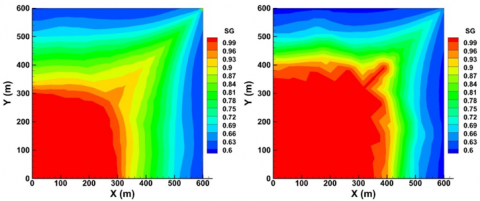
Figures 5 and 6 show the temperature and gas saturation of the reservoir after 30 years of system operation, respectively. There is a huge difference in temperature between the wellbore-reservoir coupling model and the simple reservoir model, owing to the series of thermodynamic processes of CO2 in the wellbore. By the wellbore-reservoir coupling model, the CO2 almost reached 80 °C at the bottom. Moreover, the wellbore-reservoir coupling model output a higher saturation than the simple reservoir model. This is because the CO2 density decreases with the growth in temperature, and the same amount of CO2 occupies a large space under a high temperature.
Figure 5. Distributions of reservoir temperature of the simple reservoir model (left) and the wellbore-reservoir coupling model (right)
Figure 6. Distributions of CO2 saturation in the reservoir of the simple reservoir model (left) and the wellbore-reservoir coupling model (right)
4.2 Analysis on mineral reactions
The mineral reaction rate has a positive correlation with temperature. The temperature variation in the reservoir may induce a huge difference in geothermal reactions. After the CO2 injection, the geothermal reactions generally obey the following law: The dissolution of CO2 in water reduces the pH, turning the solution acidic. Then, the calcite and feldspar are dissolved, while quartz, clay and some carbonates are precipitated.
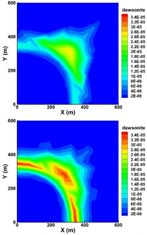
Figure 7 presents the variation in the volume fractions of dawsonite, as predicted by the wellbore-reservoir coupling model and the simple reservoir model. Dawsonite is an important carbon-fixing mineral, and a key indicator of CO2 gas reservoir. A high temperature is more favorable for the formation of dawsonite. As shown in Figure 7, both models predicted a low total volume of dawsonite, but differed greatly in the magnitude of volume variation.
Ankerite is another important carbon-fixing mineral. Compared with dawsonite, ankerite can form easily under high temperature in the gas-water two-phase mixed zone near the production well. As shown in Figure 8, the wellbore-reservoir coupling model and the simple reservoir model predicted similar distributions of ankerite, with a slight difference in the gas-water interface. Moreover, the wellbore-reservoir coupling model estimated a higher temperature and more precipitation of ankerite than the other model.
Figure 7. The variation in the volume fractions of dawsonite of the simple reservoir model (left) and the wellbore-reservoir coupling model (right)
Figure 8. The variation in the volume fractions of ankerite of the simple reservoir model (left) and the wellbore-reservoir coupling model (right)
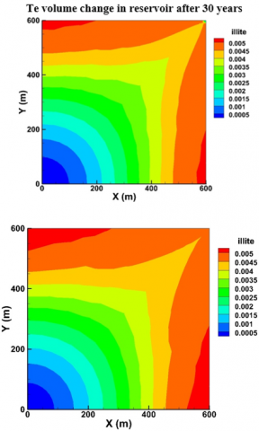
In the geochemical reactions, the dissolved species were mainly feldspar minerals like potassium feldspar (Figure 9) and anorthite (Figure 10), and the precipitated species were mainly clay minerals like illite (Figure 11), sodium montmorillonite (Figure 12) and some carbonates (Figure 13). The wellbore-reservoir coupling model output similar dissolution and precipitation situation as the simple reservoir model, except a slightly more violent dissolution and precipitation reactions near the production well. The two models predicted basically the same results in the region near the injection well, despite the huge temperature difference. In this region, the water has been displacement by CO2 or dissolved in gaseous CO2. The pure CO2 cannot react easily with the rocks.
Figure 9. The variation in the volume fractions of potassium feldspar of the simple reservoir model (left) and the wellbore-reservoir coupling model (right)
Figure 10. The variation in the volume fractions of anorthite of the simple reservoir model (left) and the wellbore-reservoir coupling model (right)
Figure 11. The variation in the volume fractions of illite of the simple reservoir model (left) and the wellbore-reservoir coupling model (right)
Figure 12. The variation in the volume fractions of sodium montmorillonite of the simple reservoir model (left) and the wellbore-reservoir coupling model (right)
4.3 Analysis on CCS amount
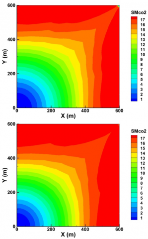
Figure 13 compares the CCS amounts (kg/m3) per unit volume of minerals in the reservoir of the wellbore-reservoir coupling model and the simple reservoir model. It can be seen that the wellbore-reservoir coupling model captured and stored more CO2 near the production well than the other model, thanks to the coexistence of gas and water and the relatively high temperature.
Figure 13. The CCS amounts per unit volume of minerals in the reservoir of the simple reservoir model (left) and the wellbore-reservoir coupling model (right)
As shown in Figure 14, the wellbore-reservoir coupling model predicted a slightly higher CCS amount than the other model. The possible reason is that a high temperature, a key parameter of geochemical reactions, speeds up the chemical reactions, enhancing the CCS ability.
Figure 14. The time variation in the total CCS amount of minerals in the reservoir of the simple reservoir model (left) and the wellbore-reservoir coupling model (right)
The wellbore is indispensable for is all geological engineering operations. Without considering the wellbore, the simple reservoir simulation will incur a huge error, failing to predict important parameters (e.g. pressure and temperature) of injection and production accurately.
Temperature is a key parameter of the geochemical reactions involving CO2. The accurate calculation of the CO2 temperature entering the reservoir helps to quantify the intensity of water-rock-gas interaction, the mineral dissolution and precipitation and the form of CCS.
Targeting a CPG project in the Songliao Basin, this paper compares the wellbore-reservoir coupling model and the simple reservoir model in terms of water and heat transfer, mineral dissolution and precipitation, change in pore permeability, and the CCS of minerals.
The comparison shows that CO2 in the wellbore varies greatly in temperature and pressure, due to its complex thermodynamic properties and flow states; the injection well is much hotter at the bottom than at the wellhead.
The mineral reactions are generally the dissolution of feldspar and precipitation of clay and carbonates. In the region near the injection well, the two models differed slightly despite the huge temperature difference, because geothermal reactions cannot occur easily without enough water. The main difference between the two models is that: the wellbore-reservoir coupling model predicted slightly more violent dissolution and precipitation reactions and a greater CCS amount near the production well than the other model.
The research findings prove the necessity of the wellbore-reservoir coupling model, laying the basis for the simulation of CO2 geological engineering.
This paper is supported by National Natural Science Foundation of China (Grant No.: 51606084), Key Science and Technology Research and Development (R&D) Project of Science and Technology Department, Jilin Province (Grant No.: 20180201078SF), Science and Technology Plan Project of Science and Technology Department, Jilin Province (Key Project of Natural Science Fund) (Grant No.: 20170101072JC) and 13th Five-Year Plan Science and Technology Project of Department of Education, Jilin Province (Grant No.: JJKH20180599KJ).
[1] IPCC (2001). The Intergovernmental Panel on Climate Change, Third Assessment Report, Cambridge University Press.
[2] Han, G., Zhang, M., Bao, L. (2012). Analysis of technical approaches and development prospect of CCUS technology. Electric Power Environmental Protection, 28(4): 8-10. https://doi.org/10.3969/j.issn.1674-8069.2012.04.003
[3] Mi, J., Mi, X. (2019). Development trend analysis of carbon capture, utilization and storage technology in China. Journal of Chinese Electrical Engineering, 39(09): 2537-2544.
[4] Zhong, P., Peng, S., Jia, L., Zhamg, J. (2011). Development of carbon capture, utilization and storage (CCUS) technology in China. China Population, Resources and Environment, 21(12): 41-45.
[5] Brown, D. (2000). A hot dry rock geothermal energy concept utilizing supercritical CO2 instead of water. Stanford University, Stanford, California, SGP-TR-165.
[6] Atrens, A.D., Gurgenci, H., Rudolph, V. (2009). CO2 thermosiphon for competitive geothermal power generation. Energy & Fuels, 23(1): 553-557. https://doi.org/10.1021/ef800601z
[7] Randolph, J.B., Saar, M.O. (2011). Coupling carbon dioxide sequestration with geothermal energy capture in naturally permeable, porous geologic formations: Implications for CO2 sequestration. Energy Procedia, 4: 2206-2213. https://doi.org/10.1016/j.egypro.2011.02.108
[8] Luo, F., Xu, R.N., Jiang, P.X. (2014). Numerical investigation of fluid flow and heat transfer in a doublet enhanced geothermal system with CO2 as the working fluid (CO2 -EGS). Energy Procedia, 64: 307-302. https://doi.org/10.1016/j.energy.2013.10.048
[9] Xu, T., Feng, G., Hou, Z., Tian, H., Shi, Y., Lei, H. (2015). Wellbore–reservoir coupled simulation to study thermal and fluid processes in a CO2-based geothermal system: identifying favorable and unfavorable conditions in comparison with water. Environmental Earth Sciences, 73(11): 6797-6813. https://doi.org/10.1007/s12665-015-4293-y
[10] Ruan, B., Xu, R., Wei, L., Ouyang, X., Luo, F., Jiang, P. (2013). Flow and thermal modeling of CO2 in injection well during geological sequestration. International Journal of Greenhouse Gas Control, 19: 271-80.
[11] Singh, A.K., Boettcher, N., Wang, W., Park, C.H., Goerke, U.J., Kolditz, O. (2011). Non-isothermal effects on two-phase flow in porous medium: CO2 disposal into a saline aquifer. Energy Procedia, 4: 3889–3895. https://doi.org/10.1016/j.egypro.2011.02.326
[12] Xu, T., Feng, G., Shi, Y. (2014). On fluid–rock chemical interaction in CO2-based geothermal systems. Journal of Geochemical Exploration, 144: 179-193. https://doi.org/10.1016/j.gexplo.2014.02.002
[13] Hangx, S.J.T., Spiers, C.P. (2009). Reaction of plagioclase feldspars with CO2 under hydrothermal conditions. Chemical Geology, 265(1-2): 88-98. https://doi.org/10.1016/j.chemgeo.2008.12.005
[14] Xu, T., Apps, J.A., Pruess, K. (2004). Numerical simulation of CO2 disposal by mineral trapping in deep aquifers. Applied Geochemistry, 19(6): 917-936. https://doi.org/10.1016/j.apgeochem.2003.11.003
[15] Xu, T., Zheng, L., Tian, H. (2011). Reactive transport modeling for CO2 geological sequestration. Journal of Petroleum Science and Engineering, 78(3-4): 765-777. https://doi.org/10.1016/j.petrol.2011.09.005
[16] Lu, M., Connell, L.D. (2014). The transient behaviour of CO2 flow with phase transition in injection wells during geological storage-Application to a case study. Journal of Petroleum Science and Engineering, 124: 7-18. https://doi.org/10.1016/j.petrol.2014.09.024
[17] Xu, T., Spycher, N., Sonnenthal, E., Zhang, G., Zheng, L., Pruess, K. (2011). TOUGHREACT Version 2.0: A simulator for subsurface reactive transport under non-isothermal multiphase flow conditions. Computers & Geosciences, 37(6): 763-774. https://doi.org/10.1016/j.cageo.2010.10.007
[18] Pan, L., Oldenburg, C.M. (2014). T2Well-An integrated wellbore–reservoir simulator. Computers & Geosciences, 65: 46-55. https://doi.org/10.1016/j.cageo.2013.06.005
[19] Shi, H., Stanford, U., Holmes, J., Geoquest, S., Durlofsky, L., Etc, C., Aziz, K., Diaz, L., Alkaya, B., Oddie, G. (2005). Drift-flux modeling of two-phase flow in wellbores. SPE Journal, 10(1): 24-33. https://doi.org/10.2118/84228-PA
[20] Pan, L., Webb, S., Oldenburg, C.M. (2011). Analytical solution for two-phase flow in a wellbore using the drift-flux model. Advances in Water Resources, 34(12), 1656-1665. https://doi.org/10.1016/j.advwatres.2011.08.009
[21] Pan, L., Oldenburg, C.M., Wu, Y., Pruess, K. (2009). Wellbore flow model for carbon dioxide and brine. Energy Procedia, 1(1): 71-78. https://doi.org/10.1016/j.egypro.2009.01.012
[22] Spycher, N., Pruess, K. (2010). A phase-partitioning model for CO2-brine mixtures at elevated temperatures and pressures: Application to CO2-enhanced geothermal systems. Transport Porous Media, 82: 173-196. https://doi.org/10.1007/s11242-009-9425-y