Omar Al-Abbasi* | Betul Sarac | Teoman Ayhan
© 2019 IIETA. This article is published by IIETA and is licensed under the CC BY 4.0 license (http://creativecommons.org/licenses/by/4.0/).
OPEN ACCESS
The humidification chamber is a vital component of the humidification-dehumidification cycle that plays an essential role in determining the effectiveness of this system. In this study, the combined effect of heating and humidifying processes in the plate type humidification chamber, the so-called solar air humidifier is investigated experimentally and using computational fluid dynamics (CFD) modeling. A lab-scale experimental setup was built consisting of a parabolic reflector coupled by a radiant heating coil, a glass plate and water tray with an insulation cover. Two parameters were investigated in the experimental phase of the study, namely, heat flux and inlet air flow rate. The mathematical model was validated against the experimental findings, and the results were in a close agreement. In addition to the heat flux and air flow rate, the effect of the height of the humidification channel was investigated theoretically. For the different heat fluxes, it has been found that the maximum evaporation rate is achieved at the smallest channel height and flow velocity. Also, the effectiveness of the humidification chamber depended strongly on the inlet conditions, and it decreased by increasing the input heat flux.
humidification-dehumidification, simulation, performance analysis, evaporation rate, desalination
With the increasing number of population and energy prices, finding new means to desalinate water is becoming an urgent need. Although, there exist several mature technologies that serve this purpose, yet the demand to have sustainable methods is pressing. Humidification-dehumidification (HDH) cycle is playing an essential role in filling this area. This technology has several features, among them is its simplicity where it is considered as the simplest cycle that operates by thermal energy [1]. Also, the low temperature operating conditions makes it a suitable cycle that can be driven using renewable energy [2-5]. The basic idea in the HDH cycle is to mix heated air with water vapor followed by water extraction from the humidified air through a condenser. The use of solar energy in HDH cycles for seawater desalination to obtain small capacity production of potable water is the subject of many investigations during recent years [6].
The performance of the HDH has been widely investigated were several researchers had proposed various methods to evaluate the performance of the whole HDH system or its subcomponents. Narayan et al., investigated the performance of several layouts of HDH cycles from the thermodynamics point of view [7]. Antar and Sharqawy carried an experimental investigation for the performance of HDH system [8]. Kalaiarasi et al., conducted energy and exergy analysis experimentally for flat plate solar air heater which is commonly used for HDH systems [9]. Abdur-Rehman et al., investigated a novel design with a multi-stage bubble column for a solar air humidifier, where the humidity had increased from 9% to 25% based on different tested conditions [10].
For a thoroughly detailed analysis of HDH cycles, computational fluid dynamics (CFD) is becoming a valuable modeling tool where it has been used by several researchers to evaluate the HDH performance. Among these studies, is the work conducted by Yadav et al., [11] where different turbulence models were evaluated in the process of designing solar air heaters, where the conclusion was that the best results are obtained using Renormalization-group k-ε model. In a similar study which is conducted by Boulemtafes-Boukadoum et al., [12], the authors studied four different turbulence closure models for a solar air heater and concluded that the SST model gives the most accurate result. Rao et al., investigated the effect of duct roughness for solar air heater using CFD modeling, where the introduced roughness has improved the effectiveness of the solar air heater significantly [13]. Another study that is related to the solar air heater was carried by Pashchenko [14]. The study investigated the optimum operating conditions for various finned configurations.
The performance of HDH system depends strongly on the effectiveness of its humidifier which is a core element the cycle. Humidifiers are classified into wetted media humidifier, ultrasonic humidifiers and spray or misting systems. For the wetted media humidifier, the rate of water evaporation from the horizontal free surface has been a subject of investigation for several researchers [15-16]. The effect of velocity, temperature, and humidity of air stream on the evaporation rate from a free surface both numerically and experimentally was conducted by Raimundo et al., [17]. The study showed that the main parameter that influences this process is velocity. For a comprehensive review of the recent advancements in HDH the reader can refer to the work done by Giwa at al., [18].
Although, the literature is rich with studies that analyze HDH, yet the parameters that affect the performance of solar air humidifier has not been thoroughly investigated. This paper aims to analyze the combined effect of heating and humidifying processes in the plate type humidification chamber, the so-called solar air humidifier (SAH) both experimentally and using CFD modeling.
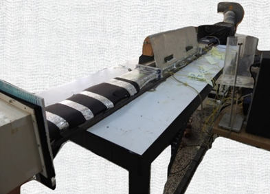
A depiction of the experimental apparatus, as well as the experimental setup, are shown in Figure 1 (a) and (b), respectively. The apparatus consists of a transition duct, test section (plate type humidification chamber), parabolic radiant heater, level controller, flow controller, and data acquisition system. A suction type duct flow is used, with dimensions of 100 mm in height, 19.6 mm in width, and 1000 mm in length, and is connected to the test section. The side walls of the duct were made of 30 mm thick fiberglass material. The test section is connected to the suction side of the fan using a channel which has the same cross-sectional area of the duct. The length of the channel is 1000 mm to avoid any turbulence at the exit of the test section through the plenum chamber.
(a)
(b)
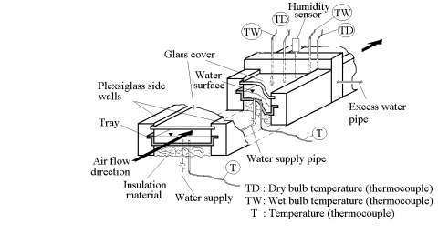
Figure 1. View of the experimental setup; (a) schematic, (b) photograph
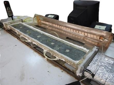
Figure 2-(a) shows a cross-section of the test section and Figure 2-(b) shows the experimental setup of the test section with the parabolic radiant heater unfolded. The test section (the plate type humidification chamber) consists of the glass cover with a 3 mm in thickness on the top surface and is heated uniformly by a parabolic radiant heater. Other sidewalls were made of acrylic plates and insulated with foam. Moreover, the bottom surface was attached to liquid water tray and insulated with silicon layers. The dimensions of the water tray are 960 mm in length, 200 mm in width, and 3 mm in depth. The water level was fixed to be 3 mm in the water tray. The gap between the upper surface and the free surface of the water layer was maintained at 3 mm. The water level during the experiments was controlled manually using the adjustable stand with a makeup water reservoir.
The parabolic radiant heater was used as a heating element to supply a uniform heat flux on the top surface of the glass cover. The resistance-heating element was installed on the focal point of the parabolic reflector. Electrical power supplied to the heating element was measured by an analogy-digital-multimeter (SO5127-1Z) that is having a measurement accuracy of ±2 %. Several power inputs were implemented in this experiment, and the power was controlled using a rheostat. Three thermocouples (K-type) were used to measure water temperature in the tray. For a better air distribution, a plenum chamber was used. An orifice plate was used for the intake air flow rate measurements using the plenum chamber, where it holds measurements to an accuracy of ±2 %. Beamex-MC5 multifunction calibrator was used to measure the differential pressure between two points, and it has an accuracy of ±1 % of reading.
(a)
(b)
For the intake air, thermocouples and humidity sensor (testo 625) with an accuracy of ±0.1 % were used to measure the air conditions. Wet and dry bulb thermocouples are pre-assembled in the plenum chamber, for comparison purposes between thermocouple and humidity sensor readings. Temperatures were recorded using a computer-based data logger. The readings of the thermocouple were stored at intervals of 5 seconds. The measurement accuracy of the thermocouple is ±0.2 °C. A mixing chamber is attached at the end of the test section, to have an even distribution measurement of the processed air. The air temperature is measured by two pairs of wet and dry thermocouples, which are being inserted at the middle of the duct height. The mixing chamber is connected to an overflow pipe as well, where it allows for the excess water to flow from the tray. Air inlet and outlet temperatures in addition to water temperature in the tray were monitored and continuously recorded. Once a steady state condition is achieved, the data acquisition system and the experiment were stopped.
The most crucial part of this experiment is to obtain accurate measurements for the rate of water evaporation. Therefore, two different methods were implemented to serve this purpose. The first method is by measuring the difference in the absolute humidity (ω) for the air stream at the inlet and the outlet of the test channel. Then the rate of evaporation ( $\dot{m}_w$ ), can be calculated according to equation (1). In this equation, three variables are needed: the mass flow rate of air ( $\dot{m}_a$ ), the air inlet humidity ratio ( w2 ), and the air outlet humidity ratio ( w1 ). In this experiment, the mass flow rate of air w2 is selected and experimentally determined (by measuring the pressure drops over the calibrated orifice plate).
$\dot{m}_w=\dot{m}_a(w_2-w_1)$ (1)
The second method which is implemented to determine the rate of evaporation is by taking the difference of the supplied water, and excess water amounts throughout each experiment. The electronic scale with an accuracy of ±0.1 g was used to measure the amounts supplied, and excess water. The uncertainty of the evaporation rate was estimated as described in [19] and it was found to be ±1.4 % for the first method and 1.9 % for the second method.
For the second method in measuring the rate of evaporation, any small error in the readings of the graduated glass vessel might result in a significant error in the volume of the water in a tray in comparison to the measured volume of the evaporated water. This was resolved by employing an excess water pipe (5-mm-dia) at the end of the tray, a stopwatch, and a 5 mm dia-plastic supply pipe which is connecting the tray and the graduated glass vessel through a valve. An adgustable stand was used to make a porper water level adjustment between the water in the vessel and water in the tray.
At the beginning of a test, the amount of the water in the vessel is weighted by the electronic scale, and the water level is marked on the vessel. During the test, a small amount of water was added slowly into the water vessel. The water flow rate could be adjusted by the valve; any overflow from the tray was also measured to provide mass balance equation of water stream. The time which water level dropped in the vessel was again marked. The difference between the two recorded times was the time required to evaporate the amount of water added because the water amounts in the tray were the same at the beginning and the end of the test.
In terms of measured quantities, the amount of added water can be expressed as a function of volume, density and time as follows:
$m ̇_v=ρ∆V/∆t$ (2)
whereρ is water density, ∆V is the change of water volume in the vessel and ∆t is the period. The relative uncertainty was found 3.2% using a mathematical correlation explained in [19]. The percentage error for the evaporation rate measured by the two methods was found to be 1.3 %.
The energy balance for the top surface of the glass cover is be given as:
$Q ̇_{gain}=Q ̇_{supply}-Q ̇_{loss}$ (3)
where$Q ̇_{gain}$ indicates the heat transfer to the air stream and water in the tray in the humidifying chamber. The electrical power source (heating element) is measured by an electronic wattmeter. $Q ̇_{loss}$ denotes electrical loss and convection loss on the top surface and conduction through the frame to the atmosphere. To estimate heat loss, the heat loss calibration was done for the heat rates of 200, 300, 400 and 500 watts. The results indicated that a heat loss of 25 % of the total supplied electrical power has occurred for the extreme conditions. The heat flux that is received by the top surface of the glass cover can be calculated as
${{q}_{flux}}=\frac{{{{\dot{Q}}}_{gain}}}{{{A}_{surface}}}$ (4)
where $A_{surface}$ is the area of the top surface of the glass cover. The effectiveness of the humidifying chamber is calculated according to the following equation:
$ε=\frac{ω_{out}-ω_{in}}{ω_{sat}-ω_{in}}$ (5)
where $ω_{out}$ is the average outlet absolute humidity from the humidifying chamber, $ω_{in}$ is the absolute humidity of the inlet air stream and $ω_{sat}$ is the saturation absolute humidity calculated at the outlet temperature.
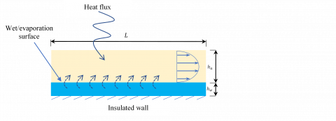
A 2d depiction of the mathematical model for the humidification chamber is shown in Figure 3 describing physical phenomena for the evaporation process. In this figure, the height of the air channel is described as ha, the height of the water tray is hw and the length of the humidification chamber is L. The air flows from left to right as shown in the laminar velocity profile. The evaporation process is taking place at the interface between the air and water surface.
Figure 3. A 2d depiction for the mathematical model
The continuity equation, i.e., mass balance, for the humid air in the chamber is given as follows:
$\frac{\partial \rho }{\partial t}+\rho \nabla \bullet u=0$ (6)
where u the velocity vector in x and y directions and ρ is the density. The Navier-Stokes equation, i.e., momentum balance, is given as:
$\rho (\frac{\partial u}{\partial t}+u\bullet \nabla u)=-\nabla p+\nabla \bullet (\mu (\nabla u+{{(\nabla u)}^{T}}))$ (7)
where p is pressure and μ is dynamic viscosity. The energy equation is written in the following form:
$\rho Cp\frac{\partial T}{\partial t}+\rho {{C}_{p}}u\bullet \nabla T+\nabla \bullet (-k\nabla T)=Q$ (8)
where Cp is specific heat at constant pressure, k is thermal conductivity, T is temperature and Q is an external heat source. The species transport for water vapor is expressed using the mass transfer equation as follows:
${{M}_{v}}\frac{\partial {{c}_{v}}}{\partial t}+{{M}_{p}}u\bullet \nabla {{c}_{v}}+\nabla \bullet (-{{M}_{v}}\nabla {{c}_{v}})=0$ (9)
where Mv is the molar mass of water vapor, D the vapor diffusion coefficient in air and Cv the water vapor concentration which can be expressed using the relative humidity ϕ and vapor saturation concentration as follows:
$c_v=ϕ c_{sat}$ (10)
The vapor saturation concentration is expressed as follows:
$c_{sat}=\frac{P_{sat} (T)}{R T}$ (11)
where R is the universal gas constant and Psat is the saturation pressure and is given as follows [20]:
${{p}_{sat}}=610.7[Pa]\bullet {{10}^{7.5\frac{T-273.15[K]}{T-35.85[K]}}}$ (12)
The boundary conditions at the inlet of the humidifying channel are given as follows:
$x=0,y=0\tilde{\ }{{h}_{a}}:{{u}_{x}}=U,T={{T}_{in}},{{c}_{v}}={{\phi }_{in}}{{c}_{sat}}$ (13)
Moreover, at the outlet of the humidifying channel, the boundary conditions are prescribed as:
$x=L,y=0\tilde{\ }{{h}_{a}}:p=0,-k\nabla T=0,-D\nabla {{c}_{v}}=0$ (14)
At the air-water interface the mass evaporation flux and heat of evaporation are expressed as follows:
$\begin{align} & x=0\tilde{\ }L,y={{h}_{w}}:\dot{m}{{''}_{w}}={{M}_{v}}k({{c}_{sat}}={{c}_{v}}) \\ & {{{\dot{Q}}}_{evp}}=-\dot{m}{{''}_{w}}{{h}_{evp}} \\\end{align}$ (15)
where $\dot{m}_{w}^{''}$ is the water evaporation mass flux, K is evaporation rate, $Q ̇_evp$ is the heat of evaporation and hevp is enthalpy of vaporization. The evaporation rate K is set to 0.1 m/s where it has been increased iteratively until the solution becomes independent of it at which water vapor is assumed to be in equilibrium with liquid water. The heat flux is applied on the upper surface of the humidifying chamber is applied as follows:
x=0~L,y=h_w+h_a: q^"=q_in (16)
The coupled system of nonlinear partial differential equations described in equations (6)-(9) are solved using COMSOL Multiphysics [21] as depicted in Figure 3. The mathematical model was solved using segregated stationary solvers with variable damping factor. The linearized systems where solved using PARDISO algorithm where the criteria for the relative tolerance was set to 1×10⁻⁴ to assure the accuracy of the solution.
A comparison between the experimental findings and the results obtained from the mathematical model are presented in Table 1, and Table 2. These results show that the model is still capable of predicting both temperature and relative humidity with a good accuracy, where the average errors are 2.5 % and 5.5 % for the temperature and the relative humidity, respectively.
A comparison between the average outlet temperature and relative humidity for low flow rates are shown in Table 1. The maximum relative error for the outlet temperature between the model and the experiment was 6 % for the case with a heat flux of 300 W. The average error for the temperature for all cases of heat flux is around 3 %. For the relative humidity, the maximum error is 8.6 % at a heat flux of 200 W, and the average error for all cases is around 4%. These results show that the model can reproduce the experiment with acceptable accuracy.
Table 2 shows a comparison between the results obtained by the model and the experimental data for the higher flow rate test, i.e., 1.2 m/s. These results show that the model is still capable of predicting both temperature and relative humidity with a good accuracy, where the average errors are 2.5 % and 5.5 % for the temperature and the relative humidity, respectively.
Table 1. Comparison between experimental measurements and numerical results at low speed (0.25 m/s)
|
Condition |
Outlet Temperature |
Relative Error in T |
Outlet Relative Humidity |
Relative Error in $\phi$ |
||
|
Texp |
Tmodel |
${{\phi }_{\exp }}$ |
${{\phi }_{\bmod el}}$ |
|||
|
200 [W] |
35.5 |
34.8 |
2.1% |
0.486 |
0.444 |
8.6% |
|
300 [W] |
40.9 |
43.3 |
6.0% |
0.384 |
0.362 |
5.8% |
|
400 [W] |
52.3 |
51.8 |
1.0% |
0.309 |
0.304 |
1.6% |
|
500 [W] |
61.1 |
60.1 |
1.6% |
0.259 |
0.262 |
1.2% |
Table 2. Comparison between experimental measurements and numerical results at high speed (1.2 m/s)
|
Condition |
Outlet Temperature |
Relative Error in T |
Outlet Relative Humidity |
Relative Error in $\phi$ |
||
|
Texp |
Tmodel |
${{\phi }_{\exp }}$ |
${{\phi }_{\bmod el}}$ |
|||
|
200 [W] |
24.5 |
24.2 |
1.2 % |
0.529 |
0.497 |
6.0 % |
|
500 [W] |
34.2 |
35.5 |
3.8 % |
0.327 |
0.343 |
4.9 % |
In this study, several parameters that affect the effectiveness of a humidifier chamber are studied. These parameters are the inlet velocity (U), air channel height (ha), input heat flux (qin) and inlet temperature (Tin) and relative humidity(${{\phi }_{in}}$). Two climate conditions, summer and winter, are considered. For the summer season, an inlet temperature of 40 °C and 60 % relative humidity and for the winter season, an inlet temperature of 25 °C and 40 % relative humidity are chosen. These conditions are picked as an average value that is resembling a meditation climate. The four inlet velocities are studied; 0.5, 1, 1.5 and 2 m/s. Three different channel heights were selected for this study; 5, 10 and 15 mm. Heat fluxes of 200, 400, 600 and 800 W/m2 were applied to match the solar irradiation.
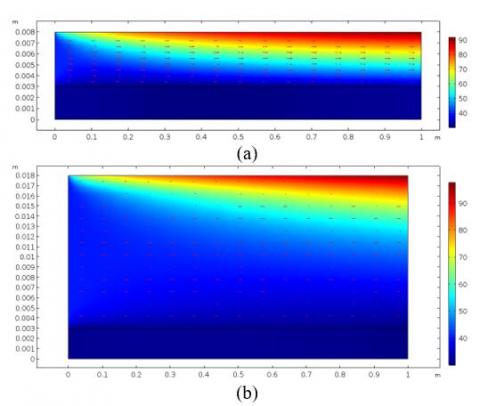
Figure 4. Temperature profile (°C) for summer conditions with a heat flux of 800 W/m2, inlet velocity of 2 m/s and air channel height of (a) 5 mm and (b) 15 mm
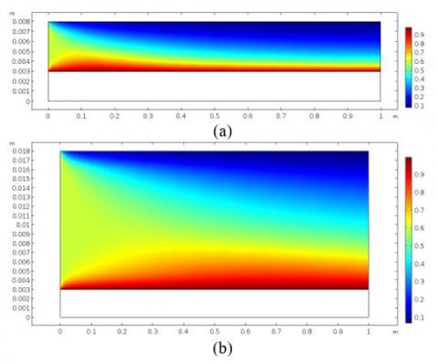
Figure 5. Relative humidity profile for summer conditions with a heat flux of 800 W/m2, inlet velocity of 2 m/s and air channel height of (a) 5 mm and (b) 15 mm
Figure 4 and Figure 5 show sample results from the numerical simulation for the temperature field and relative humidity in the humidifying chamber. The temperature distribution for the summer conditions at an inlet velocity of 2 m/s is shown in Figure 4 for two channel heights 5 mm and 15 mm, respectively. Two driving potentials are affecting the temperature in the channel, the heat flux, and the evaporation rate. The heat flux tends to increase the temperature in the channel, while the evaporation tends to decrease it. The convection heat transfer coefficient in the narrow channel is higher in comparison to the large channel leading to a higher temperature of the air stream.
Figure 5 shows a distribution of the relative humidity for the same summer conditions discussed earlier. The average outlet relative humidity for the 5 mm channel is 32 % in comparison to 44 % in the 15 mm channel. This result clearly follows the trend of the temperature distribution which is mentioned in Figure 4, where higher temperature causes a reduction in the relative humidity.
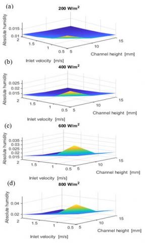
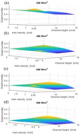
The outlet absolute humidity from the humidifying channel for summer and winter conditions are shown in Figure 6 and Figure 7, respectively. The two figures show a similar trend, where the maximum w is obtained for the smallest channel height and minimum velocity, i.e., 5mm and 0.5 m/s. These figures show an expected behaviour for the evaporation rate, where increased by increasing the heat flux. Increasing the flow velocity affected the evaporation process negatively, where increasing U decreased w, i.e., evaporation rate. The effect of velocity became more noticeable at higher heat fluxes. For example, for the channel height of 5 mm, increasing the velocity from 0.5 to 2 m/s decreased w 11.4 % at 200 W/m2. While, for the same conditions, w dropped 40 % at 800 W/m2.
Figure 6. Outlet absolute humidity of the humidifying chamber at different heat fluxes as a function of inlet velocity and channel height for summer conditions; (a) heat flux of 200 W/m2, (b) heat flux of 400 W/m2, (c) heat flux of 600W/m2, heat flux of 800 W/m2
The absolute humidity of the humidified air at the outlet of the channel decreased on average 23 % for the winter season. Again, the maximum ω was obtained for the narrowest channel and lower flow rate case, i.e., 5 mm and 0.5 m/s.
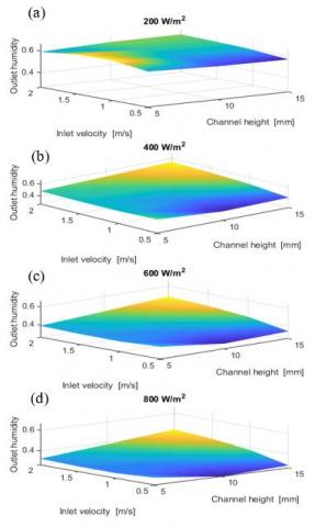
Although that the relative humidity does not reflect the evaporation rate, yet it indicates how the flow is approaching its maximum humidification potential. Therefore, the outlet relative humidity for summer and winter seasons is indicated in this study in Figure 8 and Figure 9, respectively. As expected, increasing qin tends to increase Tout as discussed in Figure 4, which eventually decreases ${{\phi }_{out}}$. One observation that can be made from these results is that for narrow channels the flow velocity has a minute effect on the outlet humidity, as the flow in this case has very small contact period to absorb the moisture. Thus, increasing the velocity did not enhance the evaporation rate. On the other hand, for larger channels, i.e., ha >10 mm, ${{\phi }_{out}}$ became more sensitive to the flow velocity. At higher heat fluxes, the maximum ${{\phi }_{out}}$ is obtained for largest channel height and flow velocity, i.e., 15 mm and 2 m/s. This means that the flow has less capacity to absorb water vapor and thus it coincides with the findings that are discussed in Figure 6 and Figure 7.
The outlet relative humidity at different heat fluxes for winter condition is shown in Figure 9. ${{\phi }_{out}}$ is noticeably smaller in winter in comparison to the summer season, as lower temperatures result in lower relative humidity. In a similar trend to summer condition, increasing U increased ${{\phi }_{out}}$, especially for larger channels. Also, increasing ${{\phi }_{out}}$ had two different effect on ${{\phi }_{out}}$ , where ${{\phi }_{out}}$ increased at high U and decreases at low U.
Figure 7. Outlet absolute humidity of the humidifying chamber at different heat fluxes as a function of inlet velocity and channel height for winter conditions; (a) heat flux of 200 W/m2, (b) heat flux of 400 W/m2, (c) heat flux of 600 W/m2, heat flux of 800 W/m2
Figure 8. Outlet relative humidity of the humidifying chamber at different heat fluxes as a function of inlet velocity and channel height for summer conditions; (a) heat flux of 200 W/m2, (b) heat flux of 400 W/m2, (c) heat flux of 600 W/m2, heat flux of 800 W/m2
Figure 9. Outlet relative humidity of the humidifying chamber at different heat fluxes as a function of inlet velocity and channel height for winter conditions; (a) heat flux of 200 W/m2, (b) heat flux of 400 W/m2, (c) heat flux of 600 W/m2, heat flux of 800 W/m2
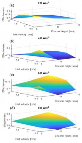
Figure 10. Effectiveness of the humidifying chamber at different heat fluxes as a function of inlet velocity and channel height for summer conditions; heat flux of 200 W/m2, 400 W/m2, 600 W/m2 and 800 W/m2
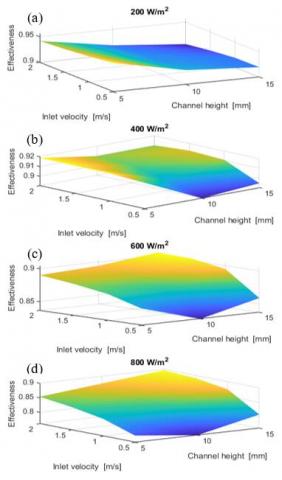
Figure 11. Effectiveness of the humidifying chamber at different heat fluxes as a function of inlet velocity and channel height for winter conditions; heat flux of 200 W/m2, 400 W/m2, 600 W/m2 and 800 W/m2
The effectiveness (ε) of the humidifying chamber for summer and winter conditions is presented in Figure 10 and Figure 11, respectively. First, it is noticed that the highest ε of the humidifying chamber does not occur at specific conditions, i.e., specific flow velocity and channel height, but it depends on the applied heat flux. At lower qin , i.e., 200 to 400 W/m2, the maximum ε was achieved at the smallest ha and U, while for higher qin , maximum ε corresponds to the largest ha and U. Second, for all the applied qin the maximum ε was achieved at the minimum heat flux of 200 W/m2 and ε decreased by increasing the heat flux. This result can be explained using equation (5), where although ω at the exit increased by increasing qin, yet the rate of increment for wsat was higher.
For winter condition, it is noticed that the trend follows the summer one. Also, the humidifying channel has higher ε in comparison to the summer condition, since the difference between ω at the exit and wsat is decreasing when the temperature is dropping.
A humidifying chamber was tested experimentally at specific dimensions and different operating conditions. A mathematical model to assess the performance of the humidifying chamber was developed and validated against the experimental findings. The model shows a good agreement with the experimental results. Several parameters: channel height, inlet velocity, heat flux, that are affecting the performance of the evaporation process in the humidifying chamber have been studied.
The highest evaporation rate was achieved for the narrowest channel and lowest flow rate, i.e., 5 mm and 0.5 m/s. The behavior of the outlet relative humidity followed a saddle surface at high heat fluxes, i.e., 400 to 800 W/m2. The maximum ${{\phi }_{out}}$ is achieved at either low U and narrow ha or large U and large ha . The effectiveness of the humidifying chamber strongly depends on the inlet conditions. At lower heat fluxes, i.e., 200 to 400 W/m2, the maximum ε was achieved at the smallest ha and U, while for higher heat fluxes, maximum ε corresponded to largest ha and U.
This work can be further extended by introducing fins in the humidification channel, where the effect of different configurations can be evaluated. Another point that is also worth investigating is the effect of the phase changing material on the effectiveness of the process and whether including such materials in the humidification channel is feasible or not.
|
A |
area, m2 |
|
c |
mole fraction of water vapor, mol/m3 |
|
CFD |
computation fluid dynamics |
|
Cp |
specific heat capacity at constant pressure, J/kg/K |
|
D |
diffusion of water vapor, m2/s |
|
h |
height of channel, m |
|
hevp |
enthalpy of vaporization, J/kg |
|
HDH |
humidification and dehumidification |
|
HH |
heating and humidification |
|
k |
thermal conductivity |
|
K |
evaporation rate, m/s |
|
L |
channel length, m |
|
$\dot{m}$ |
mass flow rate, kg/s |
|
$m^{\prime \prime}$ |
mass flux, kg/m2 s |
|
Mv |
molar mass, g/mol |
|
p |
pressure, Pa |
|
Q |
heat source, W/m3 |
|
$\dot{Q}_{evp}$ |
heat of vaporization, W |
|
R |
universal gas constant, J/K/mol |
|
SAH |
solar air humidifier |
|
T |
temperature, °C |
|
t |
time, s |
|
u |
velocity vector, m/s |
|
U |
inlet velocity, m/s |
|
Greek symbols |
|
|
ε |
effectiveness of the system |
|
η |
efficiency of the fan |
|
μ |
dynamics viscosity, Pa.s |
|
ϕ |
relative humidity |
|
ρ |
density, kg/m3 |
|
ω |
absolute humidity, kg water vapor/kg dry air |
|
Subscripts |
|
|
A |
air channel |
|
dew |
dew point |
|
evp |
evaporation |
|
In |
inlet |
|
out |
outlet |
|
sat |
saturation condition |
[1] Abdullah AS, Essa FA, Omara ZM, Bek MA. (2018). Performance evaluation of a humidification–dehumidification unit integrated with wick solar stills under different operating conditions. Desalination 441: 52–61. https://doi.org/10.1016/j.desal.2018.04.024
[2] Bourouni K, Chaibi MT, Tadrist L. (2001). Water desalination by humidification and dehumidification of air: State of the art. Desalination 137: 167–76. https://doi.org/10.1016/S0011-9164(01)00215-6
[3] Narayan GP, Sharqawy MH, Summers EK, Lienhard JH, Zubair SM, Antar MA. (2010). The potential of solar-driven humidification-dehumidification desalination for small-scale decentralized water production. Renew Sustain Energy Rev 14: 1187-201. https://doi.org/10.1016/j.rser.2009.11.014
[4] Karhe YB, Walke PV. (2013). A solar desalination system using humidification- dehumidification process- a review of recent research. Pdfs Semantic scholar Org 3: 962–9.
[5] Parekh DB, Pathan TN, Asfakbeg MH, Mirza MH, Chavda SD. (2016). A review of solar air heater with Close Water Open Air (CWOA) for humidification-dehumidification process. Int J Adv Eng Res Dev 3: 4-14.
[6] Summers EK, Lienhard JH, Zubair SM. (2011). Air-heating solar collectors for humidification-dehumidification desalination systems. J Sol Energy Eng 133: 011016. https://doi.org/10.1115/1.4003295
[7] Narayan GP, Sharqawy MH, Lienhard V JH, Zubair SM. (2010). Thermodynamic analysis of humidification dehumidification desalination cycles. Desalin Water Treat 16: 339-53. https://doi.org/10.5004/dwt.2010.1078
[8] Antar MA, Sharqawy MH. (2013). Experimental investigations on the performance of an air heated humidification-dehumidification desalination system. Desalin Water Treat 51: 837-43. https://doi.org/10.1080/19443994.2012.714598
[9] Kalaiarasi G, Velraj R, Swami MV. (2016). Experimental energy and exergy analysis of a flat plate solar air heater with a new design of integrated sensible heat storage. Energy 111: 609-19. https://doi.org/10.1016/j.energy.2016.05.110
[10] Abd-ur-Rehman HM, Al-Sulaiman FA. (2016). An experimental investigation of a novel design air humidifier using direct solar thermal heating. Energy Convers Manag 127: 667-78. https://doi.org/10.1016/j.enconman.2016.09.053
[11] Yadav AS, Bhagoria JL. (2013). Heat transfer and fluid flow analysis of solar air heater: A review of CFD approach. Renew Sustain Energy Rev 23: 60-79. https://doi.org/10.1016/j.rser.2013.02.035
[12] Boulemtafes-Boukadoum A, Benzaoui A. (2014). CFD based analysis of heat transfer enhancement in solar air heater provided with transverse rectangular ribs. Energy Procedia 50: 761-72. https://doi.org/10.1016/j.egypro.2014.06.094
[13] Rao V, Gupta A, Kumar A. (2015). CFD based heat transfer analysis of solar air. IjserOrg 6: 28-35.
[14] Pashchenko DI. (2018). ANSYS fluent CFD modeling of solar air-heater thermoaerodynamics. Appl Sol Energy 54: 32–9. https://doi.org/10.3103/S0003701X18010103
[15] Haji M, Chow LC. (1998). Experimental measurement of water evaporation rates into air and superheated steam. J Heat Transfer 110: 237-42. https://doi.org/10.1115/1.3250457
[16] Inan M, Özgür Atayilmaz Ş. (2017). Experimental investigation of evaporation from a horizontal free water surface. Sigma J Eng Nat Sci ve Fen Bilim Derg 35.
[17] Raimundo AM, Gaspar AR, Oliveira AVM, Quintela DA. (2014). Wind tunnel measurements and numerical simulations of water evaporation in forced convection airflow. Int J Therm Sci 86: 28-40. https://doi.org/10.1016/j.ijthermalsci.2014.06.026
[18] Giwa A, Akther N, Housani A Al, Haris S, Hasan SW. (2016). Recent advances in humidification dehumidification (HDH) desalination processes: Improved designs and productivity. Renew Sustain Energy Rev 57: 929-44. https://doi.org/10.1016/j.rser.2015.12.108
[19] Kline SJ, McClintock FA. (1953). Describing uncertainties in single-sample experiments. Mech Eng. 75: 3-8. https://doi.org/10.1016/j.chaos.2005.11.046
[20] Webb A. (1994). Principles of environmental physics. By J. L. Monteith & M. H. Unsworth. Edward Arnold, Sevenoaks. 2nd edition, 1990. Q J R Meteorol Soc 120: 1700. https://doi.org/10.1002/qj.49712052015
[21] COMSOL Multiphysics® v. 5.3a. www.comsol.com. COMSOL AB, Stockholm, Sweden.