Narasimha Suri Tinnaluri | Jaya Krishna Devanuri*
© 2019 IIETA. This article is published by IIETA and is licensed under the CC BY 4.0 license (http://creativecommons.org/licenses/by/4.0/).
OPEN ACCESS
The current work attempts to numerically investigate the thermal transport for two-dimensional solid complex geometries with two discrete heat sources at the bottom wall. The computational grid has been developed in GAMBIT and then linked to the in-house code which is based on collocated grid based Finite Volume Method (FVM). In this study five different domains viz. square, trapezoidal, skewed, S-curve and H-curve have been considered and the thermal conductivity has been varied from 0.25 to 10 W/m K. A concept of Bejan’s heatline visualization has been considered for the analysis of thermal transport. The heatlines along with isotherms are observed to provide a better insight for the understanding of thermal transport in considered complex geometries. With the domain thermal conductivity of 0.25 W/m K the maximum hot spot temperature is noted to be 443 K (square) and minimum of 436 K (S-curve). It is observed that with the increase in thermal conductivity from 0.25 to 10 W/m K, the maximum temperature in the domain decreased by 23.71 % for skewed and 20.77 % for S-curve geometries.
heatlines, discrete heat source, thermal transport, complex solid domains, visualization, finite volume method
The understanding of thermal transport in complex geometries with discrete heat sources is of major importance. The applications include disposal of nuclear wastes, electronic circuits, geothermal areas, food processing industries and cooling of electronic components [1-5]. A thorough understanding of thermal transport in complex geometries with discrete heat source is essential in the design of above equipment. Natarajan et al. studied two-dimensional heat function within a trapezoidal cavity which is differentially heated in the vertical direction [6]. Finite element method was used to obtain isotherms, streamlines and heatlines. They observed that when Ra (Rayleigh number) =103, the heat transfer was uniform from hot wall to the cold wall. But for Ra =106, the lower left and upper right portion of the cavity were observed with higher heat transfer rates. Deng studied laminar natural convection due to discrete heat source-sink pairs in a two dimensional cavity [7]. They analyzed the influence of arrangement of sources and sinks on fluid flow and heat transport characteristics. Banerjee et al. carried out steady state simulation for natural convection with a bi-heater configuration for the analysis of passive electronic cooling [8]. Basak and Roy demonstrated natural convection in a square enclosure with insulated top wall, hot bottom wall and cold side walls [9]. It was found that heatline concept is very much needed for optimal thermal management and also helps in the understanding of the energy distribution for the food processing application to store food for a long time. Basak et al. studied heatline concept for a trapezoidal enclosure by varying Rayleigh number in the range of 103 -105 [10], Prandtl number (0.026 ≤ Pr ≤ 1000) and at various tilted angles (Φ=450, 300 and 00). It was observed that the heatlines were perpendicular to the isotherms during conduction dominant region. Mobedi et al. employed heat function equation for the visualization of convection and diffusion in a square cavity [11]. Kaluri and Basak demonstrated natural convection in square cavity with multiple distributed heat sources [12]. It was found that visualization of heatline was useful in effective utilization of thermal resources for material processing. By using finite element method, Basak et al. studied natural convection in trapezoidal enclosures by varying boundary conditions [13]. Results were presented in terms of isotherms, streamlines, heatlines, local and average Nusselt numbers for enclosures. Heatline patterns for enclosures with Dirichlet heat function boundary conditions were reported by Biswal and Basak [14]. Triveni et al. studied natural convection due to partially heated bottom in a triangular cavity filled with water by varying Rayleigh number (105≤Ra≤107) [15]. Finite volume method was used for solving the governing equations. Results were presented in terms of streamlines, isotherms and average Nusselt numbers for various positions of the heater within the enclosure. It was observed that the increase of heat transfer rate depended on increment of Rayleigh number. Das and Basak investigated discrete solar heating involving natural convection for different types of domains such as square [16], triangular and inverted triangular geometries. Isotherms, heatlines, streamlines, local and average Nusselt number for different positions of the heater within enclosure were provided. Lima and Ganzarolli made use of heatlines to analyze the conjugate heat transfer in an enclosure having internal conducting solid body [17]. It was observed that as the ratio of thermal conductivities of fluid and solid (k*) increases from 0.01 to100 the heat transfer at the solid domains was noted to decrease. Alsabery et al. documented natural convection phenomenon in a square enclosure which is filled with nanofluid with sinusoidal heating at the horizontal walls [18]. It was found that the enhancement of heat transfer rate depended on the increment of solid wall thickness. Alam et al. investigated the thermal transport in a prismatic cavity which is filled with air [5]. It was observed that the heatlines are normal to the isotherms in conduction dominant regime. Further it was mentioned that heatlines along with isotherms give better understanding of energy distribution. Ajmera and Mathur performed experimental and numerical investigation of mixed convection in a rectangular enclosure provided with ventilation ports [19]. The parameters considered for the study were 1.25≤AR≤2.5, 3224≤Re≤6579, 8.5×10⁶≤Gr≤1.03×10⁸ and Richardson number in the range of 0.21–9.58. It was observed that there is a rise in Nusselt number with increase in Reynolds number and aspect ratio. It was also noted that enhancement of heat transfer depended on the height of ventilation ports. A thorough knowledge on heat transport phenomenon in complex domain is vital in designing efficient equipment.
Roychowdhury et al. made use of FVM with non-orthogonal collocated grid to solve incompressible N-S equations [20]. Krishna et al. considered semi-staggered grid to analyze the lid driven flow through porous media in a skewed geometry [21]. Suri and Krishna developed a numerical code to analyze heat transport in complex solid geometries following FVM philosophy with non-orthogonal collocated grid [22]. Suri and Krishna analyzed the energy transfer process in complex solid domains [23]. Results were presented in terms of isotherms and heatlines for the better understanding of thermal transport.
From the above mentioned works, it can be inferred that numerous methodologies were adopted to have a better insight on heat transport characteristics in complex geometries. In these studies, the numerical analysis was performed on a specific domain for which grid is generated. The developed code in the present study is generalized such that it can read mesh data generated for complex domains in GAMBIT. Further, an in-house FVM based code is developed on a collocated grid to analyze heat transport in terms of isotherms and heatlines for the considered complex geometries.
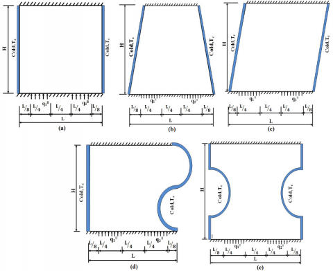
The computational domains and boundary conditions considered in the present study are shown in Figures1 (a)–(e). It consists of two-dimensional geometries of dimensions L×H. The side walls maintained at constant temperature 300K (Tc) and serve as a heat sink, two discrete heat sources are located at the bottom wall (L/4) and are maintained at constant heat flux 100 W/m2 (q1׀׀) and 200 W/m2 (q2׀׀) which serve as heat sources [24]. Other boundaries of the geometries are thermally insulated.
The governing equations for heat transport in complex domains in integral form are given as:
$∫_{∆V}\frac{∂}{∂x}(k\frac{∂T}{∂x})dxdy+∫_{∆V}\frac{∂}{∂y}(k\frac{∂T}{∂y})dxdy=0$ (1)
Diffusive flux through the east face expressed as a function of the projected areas and the values of temperature (T) at neighbouring nodes are given as:
$J_{De}=(({k_e A}_ex^1)/V_e )[{A_ex^1 (T_E-T_P )+A_ex^2 (T_ne-T_se )}]+((k_e A_ey^1)/V_e )[{A_ey^1 (T_E-T_P )+A_ey^2 (T_ne-T_se )}]$ (2)
Simplification of above Eqn. (2),
$J_De=d_e^1 (T_E-T_P )+d_e^2 (T_ne-T_se )$ (3)
where $d_e^1=k_e/V_e [(A_ex^1.A_ex^1 )+(A_ey^1.A_ey^1 )]; d_e^2=k_e/V_e [(A_ex^1.A_ex^2 )+(A_ey^1.A_ey^2 )]V_e=(x_E-x_P )(y_ne-y_se )-(x_ne-x_se )(y_E-y_P )$
Similarly, JDw, JDn and JDs can be obtained.
The net diffusive flux contribution for all sides of cell can be brought into the form
$J_D=-{d_e^1 T_E+d_w^1 T_W+d_n^1 T_N+d_s^1 T_S-(d_e^1+d_w^1+d_n^1+d_s^1 ) T_P+[b_no ]}$ (4)
where $b_no=(d_e^2+d_w^2 ) T_ne-(d_n^2+d_w^2 ) T_nw-(d_e^2+d_s^2 ) T_se-(d_w^2+d_s^2 ) T_sw$
The term bno arises as a result of non-orthogonality of the mesh which vanishes when the grid becomes orthogonal. The corner values are approximated in terms of four surrounding nodal values. For instance, the north-east corner value is given as
$T_{ne}=1/4 (T_N+T_E+T_P+T_{NE} )$ (5)
Similarly, Tnw , Tse and Tsw can be obtained.
The integral form of governing Eq. (1) over a control volume is shown in Figure 2. It may be noted that E, N, W, S, NE, NW, SE, SW represents neighbouring nodes of the control volume. e, n, w, s indicates the faces of the control volume; ne, nw, se, sw indicates corners of the control volume.1'-2'-3'-4’ indicates the auxiliary cell of control volume and is centred at face ‘e’.
Steady state heat function equation [25] can be given as
$-\frac{∂Π}{∂x}=-k\frac{∂T}{∂y}$ (6a)
$\frac{∂Π}{∂y}=-k\frac{∂T}{∂x}$ (6b)
Differentiating Eq. (6a) with respective to x and Eq. (6b) with y and by adding the equations Eq. 7 can be obtained
$\frac{∂^2 Π}{∂x^2}+\frac{∂^2 Π}{∂y^2}=0$ (7)
The boundary conditions for heatlines are obtained by integrating Eq. (7) along the boundaries at various junction points:
A reference point, $Π(0,H)=0$
is taken at the top left cornerAdiabatic top wall:$y=H;0<x≤L;$
$\prod{(x,H)=\prod{(O,H)}}-{{\int_{0}^{L}{-k\left. \frac{\partial T}{\partial y} \right|}}_{y=H}}dx=0$(8)
Cold left wall:$x=0;H>Y≥0$;
$\prod{(0,Y)=\prod{(x,H)}}-{{\int_{0}^{H}{-k\left. \frac{\partial T}{\partial x} \right|}}_{x=0}}dy$ (9)
Cold right wall:$x=1;H>y≥0;$
$\prod{(1,Y)=\prod{(x,H)}}-{{\int_{0}^{H}{-k\left. \frac{\partial T}{\partial x} \right|}}_{x=1}}dy$(10)
Adiabatic bottom wall:$y=0;0<x_a≤L⁄(8;)$
$\prod{({{X}_{a}},0)=\prod{(0,y)}}-{{\int_{0}^{L/8}{-k\left. \frac{\partial T}{\partial y} \right|}}_{y=0}}dx$ (11)
Bottom wall with heater $y=0;L⁄8<x_b<3L⁄8;$
$\prod{({{x}_{b}},0)=\prod{({{x}_{a}},H)}}-\int_{L/8}^{3L/8}{q_{1}^{''}}dx$ (12)
Adiabatic bottom wall:
$y=0;( 3L)⁄8>x_c≥5L⁄8;$$\prod{({{x}_{c}},0)=\prod{({{x}_{b}},0)}}-{{\int_{3L/8}^{5L/8}{-k\left. \frac{\partial T}{\partial x} \right|}}_{y=0}}dx$ (13)
Bottom wall with heater (q2”): $y=0;5L⁄8>x_d>7L⁄8;$
$\prod{({{x}_{d}},0)=\prod{({{x}_{c}},0)}}-\int_{5L/8}^{7L/8}{q_{2}^{*}-}dx$ (14)
Adiabatic bottom wall: $y=0;7L⁄8≥x_e>L$
$\prod{({{x}_{e}},0)=\prod{({{x}_{d}},0)}}-{{\int_{7L/8}^{L}{-k\left. \frac{\partial T}{\partial x} \right|}}_{y=0}}dx$ (15)
$d_e^1$ and $d_e^2$ denotes orthogonal and non-orthogonal diffusive fluxes for east face of the control volume respectively; $A_ex^1$ and $A_ex^2$ represents orthogonal and non-orthogonal area in x direction for the east face of the control volume.
Figure 1.Computatonal domains and boundary conditions (a) Square (b) Trapezoidal (c) Skewed (d) S curve (e) H curve
Figure 2. Typical control volume
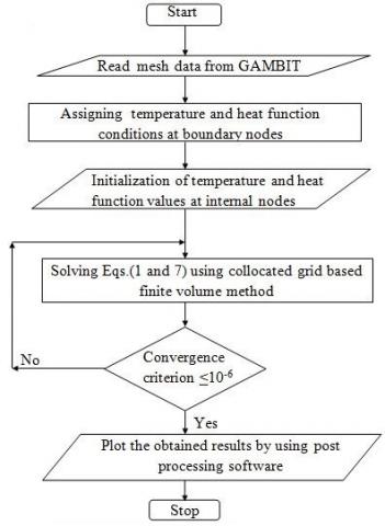
The governing Eqns (1-7) are discretized for non – orthogonal domains by using finite volume method. Numerical work has been performed for the complex domains using arbitrary quadrilateral mesh. Collocated grid arrangement is chosen which makes the terms in all the governing equations identical leading to simplified programming, minimized program storage and computational time. In this study the computational domain and its grid is generated in GAMBIT and the data is exported in neutral file format. A code in C++ is implemented to read mesh data from GAMBIT and linked to the in-house finite volume method code for the thermal transport visualization. The set of governing equations (Eqs. 1 and 7) obtained are solved using Gauss- Seidel iterative solver and a convergence criterion of 10-6 is imposed to terminate the iterations. Contour plots are used for the visualization of isotherms and heatlines for the considered geometries.
The steps considered in the present numerical methodology is provided as a flow chart and is shown in Figure 3 and can be summarised as follows
Obtained results are exported to post processing software in which contours have been plotted.
Figure 3. Flow chart for numerical methodology
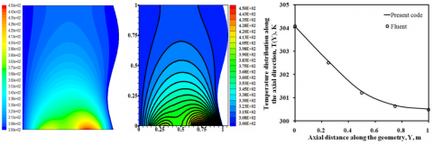
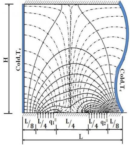
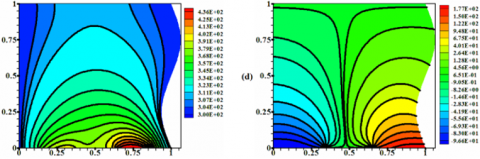
Generation of grid is important part of the numerical analysis. A numerical code in C++ has been implemented to read mesh from GAMBIT and linked to the in-house finite volume method code for the visualization of thermal transport. Grid independence has been carried out by considering mid plane temperature of the cavity. It is observed that maximum percentage variation for temperature values between grid sizes 80×80 and 120×120 is less than 1%. Therefore, a grid size of 80×80 has been considered for present study. The computational domain consists of 80 × 80 cells with 20 grid points each, on two discrete heat sources. The thermal conductivity (k) of the computational solid domains is varied between 0.25 W/m K and 10 W/m K [26]. The left hand side of the Figure 4(a) gives isotherms from commercial CFD code Ansys-Fluent and the right hand side gives isotherms from the present study. Figure 4(b) provides the quantitative comparison with Ansys-Fluent package by comparing temperature profile at mid plane. Based on Figure 4 it can be observed that the present numerical methodology is in good agreement with the commercial code Ansys-Fluent. Figure 5 shows the contours for isotherms and heatlines for the computational domain Figure 1(d). Basak et al. reported that in conduction dominant regime the isotherms and heatlines are normal to each other which can be observed from Figure 5 [27]. Based on Figures 4 and 5 it can be concluded that the present numerical methodology is validated and is in agreement with the literature.
(a) (b)
Figure 4. a) Comparison of isotherms for Ansys Fluent (left), present study (middle) and b) mid plane temperature profile with commercial CFD code (right)
Figure 5.Comparison of isotherms ( __ ) and heatlines (- - -)
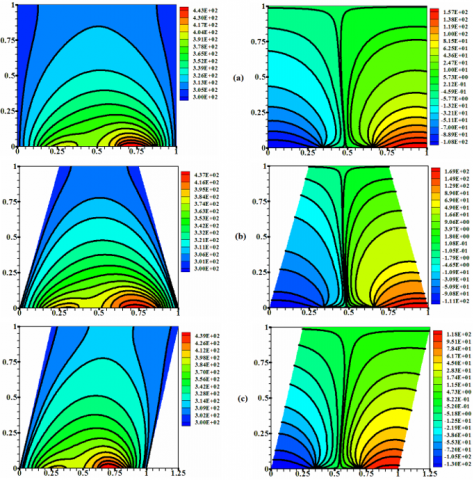
The isotherms (left), and heatlines (right) are presented in Figures 6 (a)–(e) subjected to two distinct heat sources at the bottom wall in the presence of cold side walls and insulated at the top wall. The thermal conductivity considered for the solid domains shown in Figure 6 is 0.25 W/m K. Based on the isotherms it may be noted that the magnitude of the isotherms is high at the right bottom portion of the geometries due to higher heat flux i.e. 200 W/m2 (q2׀׀) and observed to decrease as they move towards the cold side walls i.e. 300 K. Also, from the isotherms shown in Figure 6 (left) it may also be observed that they are slightly compressed towards the right bottom corner, when compared to the left bottom portion of the cavity. This phenomenon can be explained due to the position of heat flux (200 W/m2) with higher magnitude which is allocated towards the right bottom position of the cavity. This 200 W/m2 magnitude heat flux leads to the formation of hot spot with an isotherm with highest value when compared to rest of the cavity. The heat from the discrete heat sources has to be dissipated towards the cold walls which are maintained at 300 K. As the temperature gradient is more between the right portion of heat source and cold wall, the isotherms can be observed to be compressed towards right bottom of the domain. The maximum hot spot temperature for the considered geometries with thermal conductivity 0.25 W/mK is noted at the heat source q2׀׀ (200 W/m2) placed at the bottom right portion of the cavity. The maximum temperatures observed are 443 K (square), 437 K (trapezoidal), 439 K (skewed), 436 K (S-curve) and 439 K (H-curve) geometries. This behavior clearly indicates the dependence of geometry configuration on thermal transport.
The heatlines are plotted by assuming the reference point, $Π$ =0 at the top left adiabatic surface for the geometries shown in Figure 1. Based on the heatlines shown in Figure 6 (right) the heatlines move from discrete heat sources to the cold walls. As the heatlines provide the direction of heat flow, the behaviour of heatlines shown in Figures 6 (a-e) indicate the heat transport from discrete heat sources to cold walls. Also, as heat cannot dissipate through the adiabatic walls due to which the heatlines may be noted to be parallel to the adiabatic surfaces. In the present study the sign convention is based on direction of heat flow ’ $Π$ ’ from the hot to cold walls. The positive sign of ’ $Π$ ’ denotes clock wise heat flow and the anti clock wise heat flow is represented by negative sign of ’ $Π$ ’. It can be noted that the magnitude of heatlines at right wall signifies higher heat transfer rates when compared to rest of the domain. Also, the magnitude of heat function decreases from bottom heat flux portion to the central vertical axis signifying less heat transfer at that zone.
Figure 6. Isotherms (left) and heatlines (right) for different complex domains(a) Square (b) Trapezoidal (c)Skewed (d) S curve (e) H curve at k= 0.25 W/m K
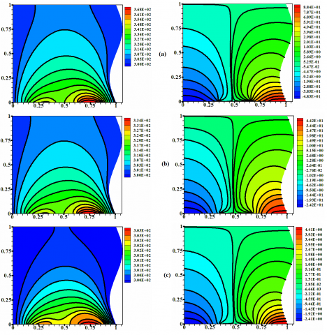
Figure 7. Isotherms (left) and heatlines (right) for S curve geometry with the variation of thermal conductivity (k) (a) 0.5 W/m K (b) 1 W/m K and (c) 10 W/m K
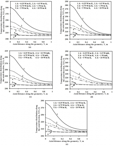
Figure 7 (a-c) illustrates isotherms and heatlines for S curve geometry with the variation of thermal conductivity (k = 0.5, 1 and 10 W/mK) at a constant heat flux condition of 100 W/m2 (q1׀׀) and 200 W/m2 (q2׀׀). Figure 6(d) represents S curve geometry with a thermal conductivity of 0.25 W/mK. It can be noted that the magnitude of isotherms decreases with the increase in thermal conductivity. This can be inferred due the increase in heat transfer due to the increase in thermal conductivity. The increase in heat transfer rate tends to the decrease in the magnitude of isotherms. In line to the decrease in magnitude of temperature, the magnitudes of the heatlines are also observed to decrease due to the decrease in temperature gradient. Figure 8 (a–e) shows the local temperature distribution along the axial direction at mid-plane drawn with the variation of thermal conductivity (k = 0.25, 0.5, 0.75, 1, 5 and 10 W/m K). Figures 8 (a) and (c), shows the magnitude of mid plane temperature higher when compared to rest of domain due to variation in size of the cavity at a thermal conductivity of k = 0.25 W/m K. When the size of the domain increases for a material whose thermal conductivity is low the heat cannot propagate and leads to higher magnitude for temperature. Also, with the thermal conductivity of k =5 and 10 W/m K the magnitude of constant temperature lines is almost same for the considered geometries. For a thermal conductivity of 0.25 W/m K the effective heat transport through the domain is less when compared to higher values of thermal conductivity. With the increase in thermal conductivity the heat transfer rate is observed to increase. The increase in heat transfer rate leads to the decrease in the magnitude of the mid plane temperature. Based on Figure 8 it can be noted that with the increase in thermal conductivity from 0.25 to 10 W/m K, the maximum temperature along the vertical mid plane for the considered domains decreased by 22.65 % (square), 20.90 % (trapezoidal), 23.71 % (skewed), 20.77 % (S-curve) and 21.35 % (H-curve) geometries
Figure 8. Variation of local temperature distribution vs axial direction along the board with different complex domains
(a) Square, (b) Trapezoidal, (c) Skewed, (d) S curve, (e) H curve
A numerical code in C++ has been implemented to read the mesh from GAMBIT and linked to the in-house finite volume method code for the visualization of thermal transport. Results are presented in terms of isotherms and heatlines for the considered geometries. The results thus obtained are compared with Ansys-Fluent. Contours for isotherms are plotted to visualize the temperature distribution and heatlines are plotted to assess the energy transport. The study could reveal that for a domain with lower thermal conductivity the magnitude of temperature increases with the increase in size. The geometry configuration is noted to influence the thermal transport. Based on results it can be observed that the visualization of heatlines provides the better insight of energy transport in domains with discrete heat sources. The study can provide an insight on the thermal management of electronic components on complex shaped circuit boards.
A projected area, m2
bno non orthogonality of the grid
d1 orthogonal part of diffusive flux
d2 non orthogonal part of diffusive flux
E,N,W,S east, north, west, south nodes
e,n,w,s east, north, west, south faces
H height in vertical direction, m
JD diffusive flux
k thermal conductivity W/m K
L length in horizontal direction, m
NE north east node
NW north west node
ne north east corner
nw north west corner
q1׀׀ left heater, W/m2
q2׀׀ right heater, W/m2
SE south east node
SW south west node
se south east corner
sw south west corner
T temperature, K
Tc temperature of cold wall, K
xa distance between left adiabatic, m
xb distance between left heater, m
xc distance between center adiabatic, m
xd distance between right heater, m
xe distance between right adiabatic, m
x, y coordinate axis
Greek symbols
$Π$ heat function W/m
△v control volume, m3
Superscripts
1 orthogonal terms
2 non orthogonal terms
[1] Krishna DJ, Basak T, Das SK. (2009). Natural convection in a non-Darcy anisotropic porous cavity with a finite heat source at the bottom wall. International Journal of Thermal Sciences 48: 1279-1293. https://doi.org/10.1016/j.ijthermalsci.2008.11.022
[2] Saravanan V, Umesh CK, Hithaish D, Seetharamu K. (2018). Numerical investigation of pressure drop and heat transfer in pin fin heat sink and micro channel pin fin heat sink. International Journal of Heat and Technology 36(1): 267-276. https://doi.org/10.18280/ijht.360136
[3] Bondarenko DS, Sheremet MA, Oztop HF, Ali ME. (2019). Natural convection of Al2O3/H2O nanofluid in a cavity with a heat-generating element. Heatline visualization. International Journal of Heat and Mass Transfer 130: 564-574. https://doi.org/10.1016/j.ijheatmasstransfer.2018.10.091
[4] Triveni MK, Panua R. (2017). Numerical analysis of natural convection in a triangular cavity with different configurations of hot wall. International Journal of Heat and Technology 35(1): 11-18. https://doi.org/10.18280/ijht.350102
[5] Alam MS, Rahman MM, Parvin S, Vajravelu K. (2016). Finite element simulation for heatline visualization of natural convective flow and heat transfer inside a prismatic enclosure. International Journal of Heat and Technology 34(3): 391-400. https://doi.org/10.18280/ijht.340307
[6] Natarajan E, Basak T, Roy S. (2007). Heatline visualization of natural convection flows within trapezoidal enclosures. In Proceedings of the 5th IASME / WSEAS International Conference on Fluid Mechanics and Aerodynamics, Athens, Greece, pp. 59-66.
[7] Deng QH. (2008). Fluid flow and heat transfer characteristics of natural convection in square cavities due to discrete source-sink pairs. International Journal of Heat and Mass Transfer 51(25-26): 5949-5957. https://doi.org/10.1016/j.ijheatmasstransfer.2008.04.062
[8] Banerjee S, Mukhopadhyay A, Sen S, Ganguly R. (2008). Natural convection in a bi-heater configuration of passive electronic cooling. International Journal of Thermal Sciences 47: 1516-1527. https://doi.org/10.1016/j.ijthermalsci.2007.12.004
[9] Basak T, Roy S. (2008). Role of “Bejan’s heatlines” in heat flow visualization and optimal thermal mixing for differentially heated square enclosures. International Journal of Heat and Mass Transfer 51: 3486-3503. https://doi.org/10.1016/j.ijheatmasstransfer.2007.10.033
[10] Basak T, Roy S, Pop I. (2009). Heat flow analysis for natural convection within trapezoidal enclosures based on heatline concept. International Journal of Heat and Mass Transfer 52: 2471–2483. https://doi.org/10.1016/j.ijheatmasstransfer.2009.01.020
[11] Mobedi M, Özkol Ü, Sunden B. (2010). Visualization of diffusion and convection heat transport in a square cavity with natural convection. International Journal of Heat and Mass Transfer 53(1-3): 99-109. https://doi.org/10.1016/j.ijheatmasstransfer.2009.09.048
[12] Kaluri RS, Basak T. (2010). Analysis of distributed thermal management policy for energy-efficient processing of materials by natural convection. Energy 35: 5093-5107. https://doi.org/10.1016/j.energy.2010.08.006
[13] Basak T, Ramakrishna D, Roy S, Matta A, Pop I. (2011). A comprehensive heatline based approach for natural convection flows in trapezoidal enclosures: Effect of various walls heating. International Journal of Thermal Sciences 50(8): 1385-1404. https://doi.org/10.1016/j.ijthermalsci.2011.03.006
[14] Biswal P, Basak T. (2015). Sensitivity of heatfunction boundary conditions on invariance of Bejan’s heatlines for natural convection in enclosures with various wall heatings. International Journal of Heat and Mass Transfer 89: 1342–1368. https://doi.org/10.1016/j.ijheatmasstransfer.2015.05.030
[15] Triveni MK, Panua R, Sen D. (2015). Natural convection in a partially heated triangular cavity with different configurations of cold walls. Arabian Journal for Science and Engineering 40: 3285–3297. https://doi.org/10.1007/s13369-015-1778-7
[16] Das D, Basak T. (2016). Role of distributed/discrete solar heaters during natural convection in the square and triangular cavities: CFD and heatline simulations. Solar Energy 135: 130-153. https://doi.org/10.1016/j.solener.2016.04.045
[17] Lima TP, Ganzarolli MM. (2016). A heatline approach on the analysis of the heat transfer enhancement in a square enclosure with an internal conducting solid body. International Journal of Thermal Sciences 105: 45-56. https://doi.org/10.1016/j.ijthermalsci.2016.02.012
[18] Alsabery AI, Chamkha AJ, Saleh H, Hashim I. (2016). Heatline visualization of conjugate natural convection in a square cavity filled with nanofluid with sinusoidal temperature variations on both horizontal walls. International Journal of Heat and Mass Transfer 100: 835-850. https://doi.org/10.1016/j.ijheatmasstransfer.2016.05.031
[19] Ajmera SK, Mathur AN. (2016). Effect of transverse aspect ratio and distinct ventilation techniques on convective heat transfer from a rectangular enclosure: experimental and numerical study. Arabian Journal for Science and Engineering 41(5): 1617-1633. https://doi.org/10.1007/s13369-015-1880-x
[20] Roychowdhury DG, Das SK, Sundararajan T. (1999). An efficient solution method for incompressible N-S Equations using non-orthogonal collocated grid. International Journal for Numerical Methods in Engineering 45: 741-763. https://doi.org/10.1002/(SICI)1097-0207(19990630)45:6<741::AID-NME601>3.0.CO;2-5
[21] Krishna DJ, Basak T, Das SK. (2008). Numerical study of lid-driven flowin orthogonal and skewed porous cavity. Communications in Numerical Methods in Engineering 24: 815-831. https://doi.org/10.1002/cnm.993
[22] Tinnaluri NS, Devanuri JK. (2015). A collocated grid based finite volume approach for the visualization of heat transport in 2D complex geometries. Procedia Engineering 127: 79-86. https://doi.org/10.1016/j.proeng.2015.11.429
[23] Tinnaluri NS, Krishna DJ. (2016). Visualization of energy transport in 2-D complex solid geometries. In IEEE, pp. 922–926. https://doi.org/10.1109/ICEETS.2016.7583880
[24] Rout SK, Thatoi DN, Acharya AK, Mishra DP. (2012). CFD supported performance estimation of an internally finned tube heat exchanger under mixed convection flow. Procedia Engineering 38: 585–597. https://doi.org/10.1016/j.proeng.2012.06.073
[25] Tao W, He Y, Chen L. (2019). A comprehensive review and comparison on heatline concept and field synergy principle. International Journal of Heat and Mass Transfer 135: 436–459. https://doi.org/10.1016/j.ijheatmasstransfer.2019.01.143
[26] Belazizia A, Benissaad S, Abboudi S. (2014). Effect of magnetic field and wall conductivity on conjugate natural convection in a square enclosure. Arabian Journal for Science and Engineering 39: 4977-4989. https://doi.org/10.1007/s13369-014-1061-3
[27] Basak T, Aravind G, Roy S. (2009). Visualization of heat flow due to natural convection within triangular cavities using Bejan’s heatline concept. International Journal of Heat and Mass Transfer 52(11-12): 2824-2833. https://doi.org/10.1016/j.ijheatmasstransfer.2008.10.034