OPEN ACCESS
The design of compact heat exchangers and their mass flow distributors is still based on empirical approaches and both experimentations and numerical analyses are needed for defining the best geometries able to reduce the mass flow rate non uniformities in parallel channels. This is a cause of reduction in both thermal and fluid-dynamic performances. In this paper, a series of single-phase and two-phase CFD simulations on water and water with air injection are carried out in order to estimate the capabilities of the solvers implemented in the OpenFOAM code to reproduce (in comparison with experimental data) such kind of configurations and phenomena. The effects of different turbulence models implemented in OpenFOAM are investigated; additionally, some general considerations on the differences and analogies among different Reynolds numbers flow and turbulence model effects applied to the present configuration are discussed. Finally, by the point of view of two-phase flow, the capability of the code to reproduce the intermittent behaviour is investigated, with the aim of obtaining an acceptable simulation of the non-uniform mass flow distribution in each protrusion; the obtained results are also compared with both ANSYS-FLUENT and STARCCM+ commercial codes.
compact heat exchangers, protrusions, parallel channels, CFD simulations, openfoam
Compact heat exchangers, such as the brazed and plate and frame types, are typically employed in refrigeration and air conditioning applications. These heat exchangers are made up of a series of stacked thermally conductive plates, creating parallel flow channels. Working as an evaporator, for example, the refrigerant fluid flows into the channels as a two phase mixture at low quality, then it evaporates and finally flows out as vapour slightly overheated. Due to the difference in inertial force, the gas and liquid phases are typically not uniformly distributed in the evaporator’s channels. The liquid separates from the gas, resulting in an uneven phase distribution throughout the heat exchanger and consequently in a loss of capacity and efficiency.
There is no general way to predict the distribution of the two-phase mixtures at the header-channel junctions. Many variables act together, such as the geometric factors (hydraulic diameter, orientation of the manifold, orientation of parallel channels connected to the manifold, intrusion depth of the channels into the header wall, length of the inlet pipe of the manifold, presence of nozzle at the inlet of the manifold) as well as the operating conditions (inlet mass flux and quality, superficial gas and liquid velocities, ratio between phase densities exit condition at downstream manifold).
Most studies on two-phase distribution in compact heat exchangers have been experimental. A literature survey is reported in Tab. 1, which includes the most important experimental parameters (geometry, experimental conditions, fluid type and protrusion depth of the channels).
The literature survey reveals that flow distribution downstream a header of a parallel flow heat exchanger is typically highly non uniform, and improvements can be obtained by inserting protruding pipes as inlet ports for the vertical channels. In most cases (downward or upward flow) the liquid distribution is significantly affected by the tube protrusion depth, but no general conclusions can be drawn.
The aim of an experimental campaign carried out in the past [14-19] was therefore to deeply investigate some phenomenological aspects of the two-phase flow separation produced by inserting protrusion tubes inside the header. The parameters of the experimentation were the protrusion depth and the gas and liquid superficial velocities. The measurements were examined in terms of the gas and liquid distributions inside the channels and comparisons were made between different configurations, including constant and variable protrusion depths.
Table 1. Experimental studies on flow distribution in header/tube configuration
|
Ref. |
Fluids |
Operating conditions |
Header / Tube configuration |
Channel flow direction (tubes) |
Diameter [mm]/ Area ratios |
Protrusion depth |
|
[1] |
Air/water |
Vsg=0 - 0.08 m/s Vsl=0.054 - 0.10 m/s |
HH square cross-section. Four vertical round pipes. Protruding type header. |
Vertical Upward |
Header A=L2 =40x40 Pipe d=10 h=0, 10, 20, 30 Abranches/Aheader = 0.196 |
0.0 ≤ h/L ≤ 0.75 |
|
[2] |
Air/water |
x =0.2- 0.5 G= 54-134 kg/m2s
Vsg=6.43 – 39.9 m/s Vsl=0.0276- 0.109 m/s |
VH square cross section. Six horizontal rectangular channels. Protruding type header. |
Horizontal
|
Header A= L2 =24x24 6 channels 22X1.8 Achannels/Aheader= 0.4126 Intrusion depth h= 0, 3, 6, 12 |
0.0 ≤ h/L ≤ 0.5 |
|
[3] |
R134a |
x=0.1- 0.35 50 to 120 kg/m2s at header |
HH circular. Protruded flat pipes (15 micro-channels). Different protrusion schemes (not uniform). |
Vertical downward |
D=20, dH=1.54 |
|
|
[4] |
Air/water |
x=0.2-0.6 70 - 130 kg/m2s
Vsg=8 – 45 m/s Vsl=0.03- 0.11 m/s |
HH circular. Vertical flat (micro-channels) tubes. Protruding type header. |
Vertical upward and downward |
D=17. 30 flat tubes. Each (micro-channel) tube has 8 rectangular ports dH=1.32 Abranches/Aheader = 0.18 |
0.0 ≤ h/D ≤ 0.5 |
|
[5] |
Air/water |
x=0.2-0.5 G= 54-134 kg/m2s
Vsg=6.43 – 39.9 m/s Vsl=0.0276- 0.109 m/s |
VH. Single or multiple side branches (T-junctions, Lee and Lee 2004)
|
Horizontal
|
D/d=7.2 Ahead/Atube =0.4, 1.6 square header 24x24 |
|
|
[6] |
R134 (21°C) |
x=0,1 to 0.4 G=130 kg/m2s
Vsg=0.44 – 1.77 m/s Vsl=0.064- 0.096 m/s |
HH. 6 downward minichannel-branches. Protrusions. |
Vertical downward |
Header D=9, 6 branches : each branch 6x0.85 i.d. Abranches/Aheader = 0.32 |
0.0 ≤ h/D ≤ 0.5 |
|
[7] |
Air/water |
x=0.2-0.6 70-200 kg/m2s |
HH circular. Vertical flat (microchannels) tubes. Protruding type header. |
Vertical upward and downward |
D=17. 10 flat tubes. Each tube 8 rectangular ports dh=1.32 Abranches/Aheader = 0.54 |
h=0.5 D |
|
[8] |
R-134a
|
70 - 130 kg/m2s x=0 .2 - 0.6 |
HH circular. Vertical minichannel tube. |
Vertical upward and downward |
D/d=12.9 AH/AT=1.9 |
h/D=0.5 |
|
[9] |
Air/water |
Vsg=7.5 – 20 m/s Vsl=0.018- 0.16 m/s |
HH circular. 2 Nozzles connected with 2 side arms. Swirl vane. |
Vertical upward arm and horizontal arm |
Header D=40 Each nozzle 8 mm, expansions angle 21°. |
|
|
[10] |
Air/water |
Vsg=0.9 – 8.8 m/s Vsl=0.35 – 0.8 m/s |
Horizontal distributor; 2 phase injection configurations; vertical test section |
Vertical upward- |
Vertical Test section: 1x1x7.13 |
|
|
[12] |
R410A |
x=0.204-0.241 341.9-1206.5 kg/h |
Plate evaporator with distributor |
Vertical upward and downward |
Ncha=24-37 Din,dist=14-28 Dh=3.18 |
|
|
[13] |
Air/water |
Vsg=0.15 – 41.70 m/s Vsl=0.005 – 0.3 m/s |
VH mixer, later splitted between 3 conducts. Vertical flat (microchannels) tubes. |
Vertical upward |
7 microchannels d=1.2 |
|
|
[14] |
Air/water |
Vsg=1.5 – 16.5 m/s Vsl=0.20 – 1.20 m/s |
HH circular. Vertical flat tubes. Protruding type header. |
Vertical upward |
D=26, df=5 Abranches/Aheader = 0.592 |
h/D=0, 0.5, 0.75, 0.9 |
LEGEND: U: mass flux [kg/m2s], x: mass quality [-]; VSL: liquid superficial velocity [m/s]; VSG: gas superficial velocity [m/s]; HH: horizontal header; VH: vertical header.
2.1 Experimental apparatus and data analysis
The experimental apparatus employed in this study is described in details in some recent papers [15-17]. The flow loop consists of a transparent test section and two supply lines of air and water, which converge into a horizontal pipe.
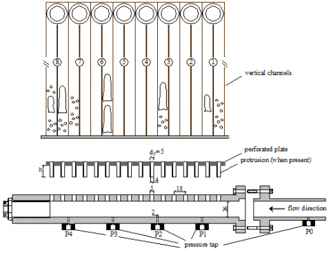
The test section (Fig. 1) consists of a horizontal distributor, which has a circular cross-section of 26 mm i.d., equipped with an interchangeable orifice plate with 16 orifices supplying an equal number of vertical channels. The channel dimensions (length, depth, width) are 500, 15, 18 mm respectively. The perforated plate has pass-through holes having a diameter (dp) equal to 5 mm; inside each of them the protruding pipes have been inserted.
Figure 1. Test section and channel pairs
Downstream of the test section, an array of valves is operated in order to extract the flow rate coming from a pair of vertical channels (channel pairs are numbered from j=1 to j=8), which carries the liquid and gas phases flow toward the corresponding flow meters.
The main and extracted (“separated”) gas streams are evaluated by two thermal mass flow meters (overall accuracy of ± 2% of the reading) and the ones for the main and extracted liquid are two magnetic devices with an overall accuracy of ±0.8% of the reading.
The gas superficial velocity is referred to the header diameter and inferred from a reference pressure and from temperature measurements (K-type thermocouples), both read just upstream the header.
Five pressure taps, named p0 to p4 along the flow direction, are connected to a differential pressure transducer and give the pressure values at the header inlet (p0), and inside it (p1 to p4).
The operating conditions, evaluated at the distributor inlet covered the following ranges of gas and liquid superficial velocities: Vsg=1.50÷16.50 m/s and Vsl=0.20÷1.20 m/s, respectively. Intermittent and annular flows were visually observed by analysing the two-phase flow structure.
Experiments were carried out by protruding the vertical channels into the header by means of short pipes (external diameter 5 mm, internal one 4 mm).
Figure 2. Variable protrusion depth configurations: (a) P3; (b) P2
These pipes have been changed initially according to 3 different configurations having a constant protrusion depth h equal to 13, 19.5 and 23.5 mm respectively. The corresponding h/D ratio is equal to 0.5, 0.75 and 0.90, respectively. Two new configurations have been here investigated: they are characterized by a variable protrusion depth along the distributor, as showed in fig. 2. In the first one (hereafter “P3”) the protrusion depth has 3 levels: it increases in the flow direction from h/D=0.50 (protrusions 1 and 2), to h/D=0.75 (protrusions 3, 4, 5 and 6), to h/D=0.90 (protrusions 7, 8, 9 and 10), then it symmetrically decreases to h/D=0.75 (protrusions 11, 12, 13 and 14) and to h/D=0.50 (protrusions 15, 16). The second configuration (hereafter “P2”) has only 2 depths: the protrusion depth is constant (h/D=0.90) except for the first 2 protrusions and the last two (protrusions 15, 16) for witch h/D=0.75.
The gas and liquid flow rates are reported in a non-dimensional way. For the generic phase k (k=g for the gas and k=l for the liquid) the dimensionless flow rate is defined as:
$\dot{m}_{k,j}^{*}=\frac{\dot{m}_{k,j}^{{}}}{\sum\limits_{i=1}^{N}{\dot{m}_{k,j}^{{}}/N}}$ (k= g, l) (1)
where N is the total number of channel pairs and j refers to the channel pair under consideration.
Another synthetic representation of the phase distributions inside the channels is the standard deviation of the k-phase flow ratio, defined as follows:
$ST{{D}_{k}}={{\sqrt{{{\sum\limits_{j=1}^{N}{\left( \dot{m}_{k,j}^{*}-1 \right)}}^{2}}/N}}^{{}}}$ (2)
that represents a single-value index of liquid which expresses the distribution / maldistribution of the flow rate of the liquid or of the gas phase.
2.2 Experimental findings
In a first step the protrusion depth was held constant along the entire header length; the 3 different configurations analysed had the dimensionless depth h/D equal to 0.50, 0.75 and 0.90 respectively.
It can be observed that the protruded pipes can exert a positive influence on phase distribution provided that the dimensionless depth h/D is greater than 0.5. In fact either the gas or liquid distribution are very similar to the “ref” case (this condition refers to the header with no fittings inside the header) when the protrusion is too short: in this case most of the gas flows inside the first channels from header inlet, while the liquid migrates to the central/end channels.
The analysis of the measurements, gathered for other liquid velocities, leads to similar conclusions, even if the effect of the protrusion depth is less apparent.
Increasing the protrusion depth, the flow distribution improves considerably, with a typical trend: the liquid ratios in the central channels (j = 4, 5 and 6) are lower than those of other channels; the gas ratios exhibit the opposite behaviour, with low values in the first and last channels.
The results discussed above suggested that, in order to decrease the liquid flow ratio in the first and last channels, the size of protrusion may be different along the distributor: a shorter protrusion depth in the initial and ending part of the header may penalize the liquid ratio in these regions, hence increasing the distribution in the central channels.
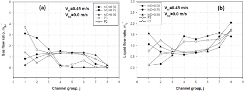
Figure 3. Gas and liquid flow ratios for different protrusion configurations, Vsl=0.45 m/s, Vsg=9.0 m/s
Figure 4. Gas and liquid flow standard deviations inside parallel channels: effect of the protrusion depth, Vsl=0.45 m/s
Fig. 3 shows the effect of the variable protrusion depth for the condition Vsl=0.45 m/s, Vsg=9.0 m/s. The behaviours of P3 and P2 configurations are very different: in the first channel P3 increases the gas flow ratio (Fig. 3(a)) and decreases the liquid flow ratio (Fig. 3(b)); at the same time liquid ratio of the last channel is significantly larger than those of other channels, yielding worse flow distribution even than with short protrusions (h/D=0.50). An excellent uniform distribution was obtained with P2 configuration: more liquid was supplied to upstream channels (Fig. 3(b)), while the gas was fairly uniformly distributed to inner channels, as for h/D=0.75÷0.90.
To quantify the flow distribution, standard deviations were calculated by Eq. (2), and are showed in Fig. 4. The graphs in Fig. 4a and 4b show the profiles of the gas and liquid standard deviations for Vsl=0.45 m/s, as a function of the gas superficial velocity. The typical trends are opposite: as the gas flow rate is increased, the gas distribution inside channels gets better, while the liquid one worsens. Inspection of Fig. 4 reveals that increasing the protrusion depth the phase standard deviations have significant benefits in comparison with the reference situation.
The liquid distribution is more uniform with the highest protrusion depth h/D=0.90 and with P2 configuration, except for the highest gas velocity. The singular behaviour of STDl for Vsg=1.5 m/s is due to the strong decrease of the liquid phase in channels 7 and 8, which leads to a less uniform flow distribution.
Similar STD profiles were also observed at higher liquid velocities (Vsl=0.80 and 1.20 m/s). Either the gas or liquid distribution are very similar or even worse to the “ref” case when the protrusion is short: in this case most of the gas flows inside the first channels from header inlet, while the liquid goes to the central/end channels. The P3 configuration has a similar behaviour, probably because the first two short protrusions are not able to catch enough liquid phase. The best observed liquid phase distribution have been obtained for P2 configuration.
3.1 OpenFOAM
One of the main aim of the present research is a first evaluation of the capabilities of some solvers implemented in an open-source CFD code (namely OpenFOAM [20]) to reproduce the configurations and the phenomena in comparison with the experimental data reported in the previous paragraphs.
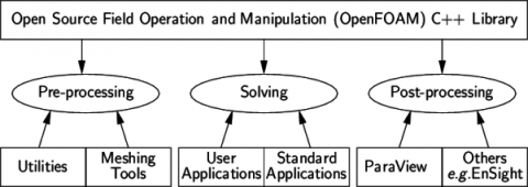
Figure 5. Overview of OpenFOAM structure [20]
As known, OpenFOAM is firstly and foremost a C++ library which must be linked together to perform the CFD analysis. The executable generated by the libraries can be classified into two main categories: the solvers, which are each designed to solve a specific problem in continuum mechanics and the utilities, which are designed for postprocessing. The OpenFOAM distribution contains numerous solvers and utilities covering a wide range of problems.
The code version used in this research is v3.0+.
3.2 CFD numerical models
The numerical study of the effect of the protrusions on the distribution of the mass flow rate into 16 channels has been performed by means of OpenFOAM with reference to the single phase flow case.
The computational domain is reported in Fig. 6: it includes the complete volume of the distributor and the 16 small pipes, which are inserted in it. The inlet section (dinlet = 26.0 mm) of the computational domain is set at the connection of the feeding pipe and the distributor. Downstream, the computational domain ends at the protrusions outlet, where they converge in bigger pipes used for collecting (in pairs) and then measuring (in ad-hoc experimental test sections) the mass flow rates flowing through the 16 channels. The axial extension of the domain is 314 mm. The grid selected for the final run has 1733984 hexahedral cells, 5267344 faces and 1800355 nodes. The minimum volume of a cell is 3.35·10-11 m³ while the maximum volume is 2.06·10-10 m³; the maximum Aspect Ratio and Skewness are, respectively, 4.5 and 0.85.
Figure 6. Computational fluid domain
The Navier-Stokes equations for a single-phase flow with a constant density and viscosity (as implemented in the OpenFOAM code [20, 21]) are the following:
$\nabla (\rho \vec{U})=0$ (3)
$\frac{\delta \overrightarrow{U}}{\delta t}+\nabla \cdot (\overrightarrow{v}\overrightarrow{v})-\nabla \cdot \left( \upsilon \nabla \vec{v} \right)=-\nabla p$ (4)
The specific solvers used for CFD simulations in the present paper are simpleFOAM (steady-state solver for incompressible, turbulent flow) and pisoFOAM (transient solver for incompressible, turbulent flow), both with different turbulence models. The main difference between these two solvers is that while pisoFOAM is a transient solver (i.e. it runs on the basis of time-steps which capture the fluctuations associated with turbulence), simpleFOAM is steady-state (i.e. it just aims to reach a converged “steady” solution in a certain number of iterations). In principle, both the kind of solvers should reach (at least on average) the same results, although a steady-state one cannot show the dynamic evolution of the considered system (e.g. the eddies formation, etc.). For further (and more general) details on the SIMPLE and PISO algorithms, see [20, 22].
Looking at the used turbulence models, for steady-state analyses we chose Standard, Realizable, RNG k-ε and SST k-ω models, while, for the transient simulations, only Standard k-ε, SST k-ω and an Isochoric LES turbulence models (namely the Spalart-Allmaras model).
3.3 Boundary conditions
Tab. 2 reports the mean velocity, which have imposed at the inlet, for the steady state analysis.
A special care has been devoted to size of near-wall cells: their size has been selected in such a way that the value of y+ would be between 34 and 50 in order to use the model "wall functions” at the wall. The outlet of the protrusion has been defined with constant pressure (set to 0 due the relative value required) together with the BCs of zeroGradient (normal gradient of the transported scalar quantity imposed zero). The velocity profile entering the domain has been implemented as fully developed turbulent flow through GroovyBC implemented in the Swak4foam tool; the chosen velocity profile was the "Power Law" [22], with exponent 7.
3.4 Grid-independency preliminary analysis
With the aim of to check independence of the results from the mesh, a sensitivity analysis test was performed. The selected case was 1530 l/h, corresponding to Re=20000; also k-ε and SST k-ω models have been tested to avoid dependence by the different wall treatment of this two turbulence models. Three different mesh sizes have been used, respectively with 1.7, 3.4 and 6.8 Mnodes, hexahedral cells, designed in order to have a difference in the wall y+ as low as possible.
Figure 7. Mesh independency test with k-ε standard model
Figure 8. Mesh independency test with k-ω SST model
Fig. 7 and 8 show the trend of the results of this test respectively with standard k-ε and k-ω SST turbulence models, and tab. 3 and 4 the average percentage differences between the results obtained by the 1.7 Mnodes grid and the refined ones.
Table 2. Selected mass flow rates
|
Mass_flow_rate [l/h] |
Average velocity at inlet [m/s] |
Re [-] |
|
860 |
0.45 |
10000 |
|
1530 |
0.80 |
20000 |
|
2300 |
1.20 |
30000 |
Table 3. Difference between 1.7, 3.4 and 6.8 Mnodes grids results with k-ε standard turbulence model
|
|
|
Difference [%] with 1.7 Mnodes |
|
|
Protrusion couple n |
1.7 Mnodes [l/h] |
3.4 Mnodes |
6.8 Mnodes |
|
I |
175.1 |
0.37% |
0.79% |
|
II |
181.5 |
0.55% |
0.45% |
|
III |
183.7 |
0.03% |
0.39% |
|
IV |
188.6 |
0.04% |
0.08% |
|
V |
195.3 |
0.20% |
0.31% |
|
VI |
201.1 |
0.20% |
0.35% |
|
VII |
203.2 |
0.02% |
0.59% |
|
VIII |
203.4 |
1.31% |
0.49% |
|
Mean difference [%] |
0.34% |
0.43% |
|
Table 4. Difference between 1.7, 3.4 and 6.8 Mnodes grids results with k-ω SST turbulence model
|
|
|
Difference [%] with 1.7 Mnodes |
|
|
Protrusion couple n |
1.7 Mnodes [l/h] |
3.4 Mnodes |
6.8 Mnodes |
|
I |
171.9 |
1.53% |
0.78% |
|
II |
178.1 |
0.64% |
0.27% |
|
III |
180.1 |
2.13% |
1.92% |
|
IV |
189.3 |
0.48% |
0.24% |
|
V |
200.6 |
3.26% |
2.51% |
|
VI |
203.4 |
1.86% |
1.67% |
|
VII |
203.3 |
0.12% |
0.02% |
|
VIII |
205.3 |
0.15% |
1.55% |
|
Mean difference [%] |
1.27% |
1.12% |
|
The results of these preliminary tests show that the differences in terms of the predicted trends and deviations are negligible when compared to the required increments in the computational efforts, for both the two tested turbulence models. For this reason, the selected mesh chosen for the simulations is the one with the lower number of nodes, i.e. 1.7 Mnodes.
4.1 Steady-state analysis
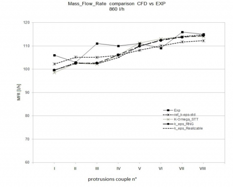
Fig. 9 shows the results obtained with the flow rate of 860 l/h; Tab. 5 reports the percentage error (with reference to the experimental conditions) obtained by the simulations. Because in the experimental facility there are only 8 mass flow meters each of them collect a couple of protrusions: for this reason the results of the CFD analysis reports the aggregate value of pairs of two consecutive protrusions (e.g. the value n. I is referred to the protrusions n. 1 and 2, the value n. II to the protrusions n. 3 and 4, etc.).
All the turbulence models predict the value of the mass flow rate evolved in each couple of protrusions with a similar average percentage error (around 3%); the minimum error corresponds to the II and VIII couples of protrusions while the maximum to the III. The results obtained by CFD calculations are very similar, and for all the models the results trends are smoothed if compared to the experimental ones; particularly, the first and the third couples of protrusions show the higher percentage errors, due to the deviation of the experimental results from a “regular” trend.
Table 5. Errors [%] at 860 l/h
|
Couple of protrusions |
k-ε (standard) |
Realizable k-ε |
RNG k-ε |
k-ω STT |
|
I |
5.7 |
6.0 |
6.1 |
7.0 |
|
II |
0.2 |
0.2 |
0.5 |
0.5 |
|
III |
6.6 |
7.8 |
7.6 |
8.0 |
|
IV |
3.7 |
4.5 |
3.5 |
3.7 |
|
V |
1.6 |
1.0 |
1.0 |
0.3 |
|
VI |
2.7 |
3.4 |
3.1 |
3.7 |
|
VII |
2.2 |
1.7 |
1.9 |
1.8 |
|
VIII |
0.9 |
0.1 |
0.6 |
0.9 |
|
Average error |
2.9 |
3.1 |
3.0 |
3.2 |
Figure 9. CFD vs. experimental mass flow rates comparison at 860 l/h
Figure 10. CFD vs. experimental mass flow rates comparison at 1530 l/h
The reasons of the smoothing in the CFD calculations could be due to the numerical “forcing” of the solver to reach a steady-state solution; the absence of the time-dependent terms could lead the solver to underestimate the effects of time-dependent instabilities and to calculate a smoother velocity field.
Fig. 10 shows the results obtained with the flow rate of 1530 l/h and Tab. 6 reports the percentage error (with reference to the experimental conditions) obtained in the simulations.
In this case, the maximum errors is placed near the inlet, probably due to the flow instabilities localized around the I and II couples of protrusions, instead very low errors are found in the last couple of protrusions. Differently from the results of the analysis at 860 l/h, the percentage errors (although higher) strongly depend on the turbulence models, which were used, and the SST k-ω model shows the highest average error, that reaches 10% in the first couple of protrusions. This error is probably determined by the complexity of the pattern of the flow impingement upon the first protrusion.
Table 6. Errors [%] at 1530 l/h
|
Couple of protrusions |
k-ε (standard) |
Realizable k-ε |
RNG k-ε |
k-ω STT |
|
I |
8.3 |
9.2 |
8.9 |
10.0 |
|
II |
3.9 |
4.8 |
5.0 |
5.8 |
|
III |
5.3 |
5.9 |
6.3 |
7.2 |
|
IV |
3.3 |
3.0 |
2.9 |
2.9 |
|
V |
0.7 |
2.8 |
1.8 |
3.4 |
|
VI |
2.1 |
2.7 |
2.7 |
3.2 |
|
VII |
3.2 |
2.8 |
3.5 |
3.2 |
|
VIII |
1.7 |
1.2 |
1.9 |
2.7 |
|
Average error |
3.6 |
4.0 |
4.1 |
4.8 |
Unlike the numerical results trend at 860 l/h, the CFD curves have a much more uneven trend than experimental ones, in particular in the I, II, III and IV couple of protrusions; additionally, in the CFD results a rising mass flow rate value in each model appears, differently from the very smooth variations of the experimental data. Similarly to the previous considerations on the steady-state solution, we have a quasi-linear increment in the mass flow rate value, without noticeable instabilities between two consecutive couple of protrusions.
Table 7. Errors [%] at 2300 l/h
|
Couple of protrusions |
k-ε (standard) |
Realizable k-ε |
RNG k-ε |
k-ω STT |
|
I |
6.0 |
6.6 |
6.7 |
8.2 |
|
II |
4.1 |
3.5 |
3.0 |
1.4 |
|
III |
5.0 |
5.1 |
6.0 |
6.8 |
|
IV |
0.6 |
0.4 |
0.3 |
0.2 |
|
V |
1.0 |
0.5 |
0.2 |
2.7 |
|
VI |
2.0 |
2.9 |
2.7 |
3.3 |
|
VII |
2.0 |
0.9 |
2.2 |
1.4 |
|
VIII |
1.2 |
1.2 |
1.6 |
2.2 |
|
Average error |
2.7 |
2.7 |
2.8 |
3.3 |
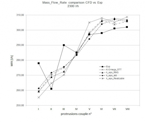
Fig. 11 shows the results obtained with a flow rate of 2300 l/h and tab. 7 reports the percentage errors (with reference to the experimental conditions) obtained in the simulations.
Figure 11. CFD vs. experimental mass flow rates comparison at 2300 l/h
In this set of simulations, the average percentage errors are very low and the profile of mass flow rates is very similar to the experimental one; like the previous showed results, there are relatively bigger errors only for the I and the III couples of protrusions. In these cases, there are very similar trends in both the numerical and experimental results; however, in the first and third couple of protrusions experimental instabilities of the mass flow rate distributions (unseen in the CFD results) appears. In the last three couples of protrusions the SST k-ω and the RNG k-ε models show uneven trends; particularly, in the VII protrusions couple there is a lower mass flow rate value than those in the surrounding couples of protrusions couple (i.e. VI and VIII); this behaviour is similar to that one experimentally measured in the II and IV protrusions couples.
4.2 Transient Analysis
A further set of simulations, by means of pisoFOAM transient solver, has been performed In order to evaluate the effect of time-dependent instabilities on the extent of maldistribution of the mass flow rate. The imposed BCs are obviously the same already adopted for the simulations by simpleFOAM solver. For the LES based solver two different grids (respectively composed by 1.7 and 3.4 M of cells) have been tested.
The obtained results are reported in fig. 12, 13 and 14 and Tab. 8, 9 and 10, respectively for 860, 1530 and 2300 l/h tests.
Table 8. Errors [%] at 860 l/h (transient solver)
|
Couple of protrusions |
k-ε |
k-ω SST |
|
I |
0.2% |
0.6% |
|
II |
4.0% |
3.5% |
|
III |
3.9% |
5.1% |
|
IV |
3.1% |
4.3% |
|
V |
3.3% |
3.6% |
|
VI |
0.6% |
0.2% |
|
VII |
5.4% |
4.7% |
|
VIII |
4.7% |
2.3% |
|
Average error |
3.15% |
3.05% |
Table 9. Errors [%] at 1530 l/h (transient solver)
|
Couple of protrusions |
k-ε |
k-ω SST |
|
I |
2.8% |
3.9% |
|
II |
0.3% |
0.7% |
|
III |
2.6% |
3.7% |
|
IV |
2.9% |
4.1% |
|
V |
1.3% |
1.7% |
|
VI |
1.5% |
1.2% |
|
VII |
0.5% |
0.8% |
|
VIII |
1.5% |
1.6% |
|
average error |
1.7% |
2.2% |
Table 10. Errors [%] at 2300 l/h (transient solver)
|
Couple of protrusions |
k-ε |
k-ω SST |
|
I |
0.7% |
1.8% |
|
II |
8.5% |
7.5% |
|
III |
2.5% |
3.2% |
|
IV |
0.4% |
1.1% |
|
V |
2.9% |
2.9% |
|
VI |
1.7% |
1.5% |
|
VII |
1.4% |
0.5% |
|
VIII |
1.0% |
1.0% |
|
average error |
2.4% |
2.4% |
Figure 12. CFD vs. experimental mass flow rates comparison at 860 l/h (transient solver)
Figure 13. CFD vs. experimental mass flow rates comparison at 1530 l/h (transient solver)
Figure 14. CFD vs. experimental mass flow rates comparison at 2300 l/h (transient solver)
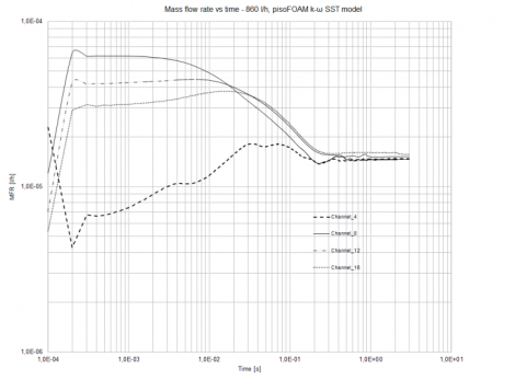
All the simulations have achieved stationary values after 1÷1.5 s, as it can be seen in Fig. 15.
Fig. 15 shows the temporal trend of the mass flow rate detected through the channel 4, 8, 12 and 16 at 860 l/h and with SST k-ω model (all the transient simulations showed similar results
The results of the transient analysis, at 860 and 2300 l/h, do not give a substantial reduction in the mean error trends, in comparison with the steady state analysis presented in the previous paragraph.
Figure 15. Mass flow rate temporal trends at 860 l/h (k-ω SST turbulence model)
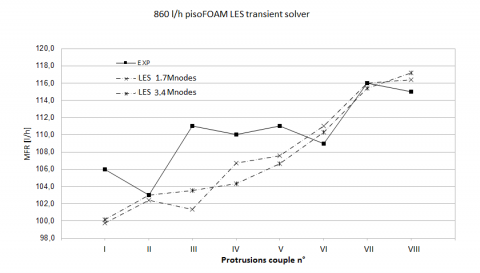
Figure 16. CFD vs. experimental mass flow rates comparison at 860 l/h with LES turbulence model (transient solver)
However, some interesting results were obtained at 1530 l/h: in addition to a very low average percentage errors, the mass flow rate distribution with both turbulence models seems virtually specular to the experimental one, between the II and V protrusions couples (in particular with the SST k-ω turbulence model). Similar results have been obtained with the LES Spalart-Allmaras isochoric turbulence model with 1.7 Mnodes at 860 l/h (Fig. 16): in this case, the virtually specular (to the experimental data) trend was obtained between I and VI protrusions couples.
Despite the (relatively) high percentage errors (see Tab. 10 and 11) in the specular part, the transient pisoFOAM k-ω solver and the pisoFOAM Spalart-Allmaras isochoric LES model can predict an instable behaviour, unlike the other tested models.
Table 10. Errors [%] at 2300 l/h (transient solver)
|
Couple of protrusions |
k-ε |
k-ω SST |
|
I |
0.7% |
1.8% |
|
II |
8.5% |
7.5% |
|
III |
2.5% |
3.2% |
|
IV |
0.4% |
1.1% |
|
V |
2.9% |
2.9% |
|
VI |
1.7% |
1.5% |
|
VII |
1.4% |
0.5% |
|
VIII |
1.0% |
1.0% |
|
average error |
2.4% |
2.4% |
Table 11. Errors [%] at 860 l/h (transient solver with LES)
|
Couple of protrusions |
LES |
LES_ref1 |
|
I |
5.9% |
5.5% |
|
II |
0.6% |
0.0% |
|
III |
8.7% |
6.7% |
|
IV |
3.0% |
5.2% |
|
V |
3.1% |
3.9% |
|
VI |
1.9% |
1.2% |
|
VII |
0.0% |
0.5% |
|
VIII |
1.2% |
1.9% |
|
average error |
3.0% |
3.1% |
The tested RANS steady solvers require a relative short time to reach convergence; the k-ω model based calculations are the fastest, although all the steady-state RANS turbulence models tested do not exceed 3 hours in the calculations times (Tab. 12), with very low percentage errors in comparison to the experimental data.
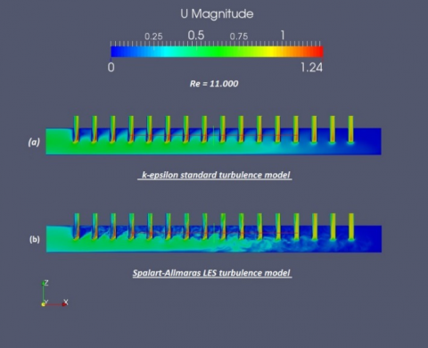
On the contrary, with the transient simulations (including LES based ones), although there is definite improvement in the turbulent and chaotic flow representations inside the computational domain (e.g. by the resolution of large eddy structures, see Fig. 17), the evaluation of mass flow rate is only slightly improved. In particular, it is possible to predict the instabilities of the profiles of mass flow rate distributions but with the calculation time increases by a factor 7 or more.
Table 12. CPU times for parallel calculations with 4 cores (Intel I7-5960X)
|
Model |
CPU time [s] |
|
simpleFoam_k-ε |
9065 |
|
simpleFoam_k-ω |
8590 |
|
pisoFoam-RAS |
60710 |
|
pisoFoam Spalart-Allmaras |
69794 |
Figure 17. Comparison of turbulent flow fields predicted by (a) RANS k-ε (standard) and (b) LES Spalart-Allmaras models
A CFD analysis of a multiport distributor has been accomplished and results were compared with available experimental data. The results shows a good agreement with the experimental data, with very low deviations which, in the worst case, do not reach the 10% for a single protrusions couple and 5% (as an averaged value) for all the protrusions couples. Furthermore, many different turbulence models have been used and they did not show any significant differences from the point of view of both the percentage deviations and the distribution profiles in steady-state solutions; the transient solvers show in some case a good prediction of mass flow distribution trend, without appreciable improving of the accuracy and increasing the calculation time by a factor larger than 7. Substantially the tested LES turbulence model does not lead to an appreciable improvement in the results; on the contrary we note a significant increase in the calculations times.
Then we can say that OpenFOAM predicts properly mass flow rates distributions (at least in the analysed range of Reynolds numbers).
This preliminary code-to-experiment comparison has provided very interesting results, also in view of a future further development of numerical models able to simulate even multiphase flow distributions within the different protrusions. Then, as a further future potential development, it could be also possible to (even only) computationally optimize (in terms of flow distribution uniformity) the collector geometrical configuration.
Our first thank goes to Prof. M. Fossa of DIME/TEC (University of Genova) for the invaluable support provided during the experimental research activity upon which this paper is based. Special thanks to Ing. D. Chersola of DIME/TEC (University of Genova) and Dr. R. Marotta of Nucleco S.p.A. for their help and suggestions. Finally we want to thank Ing. F. Magugliani of Ansaldo Nucleare S.p.A. for his help in solving computational issues.
|
µ |
Dynamic viscosity, [Pa∙s] |
|
ρ |
Density, [kg/m3] |
|
k |
Turbulent kinetic energy, [m2/ s2] |
|
ε |
Turbulence dissipation, [m2/ s3] |
|
ω |
Turbulence dissipation rate, [s-1] |
|
A |
Surface, [m2] |
|
D |
Diameter, [m] |
|
H |
Height, [m] |
|
MFR; ṁ |
Mass Flow Rate, [kg/s] |
|
VFR |
Volumetric Flow Rate, [m3/h] |
|
N |
number of channels pairs |
|
p |
Pressure, [Pa] |
|
v |
Velocity, [m/s] |
|
L |
Length, [m] |
|
Pr |
Prandtl number |
|
Re |
Reynolds number |
|
STD |
STandard Deviation |
[1] Horiki S., Osakabe M. (1999). Water flow distribution in horizontal protruding-type header contaminated with bubbles, Proceeding of the ASME Heat Transfer Division, Vol. 2, pp. 69-76. DOI: 10.1016/S0301-9322(98)00067-6
[2] Lee J.K., Lee S.Y. (2004), Distribution of two phase annular flow at header-channel junctions, Exp. Thermal and Fluid Science, Vol. 28, pp. 217-222. DOI: 10.1016/S0894-1777(03)00042-6
[3] Bowers C.D., Hrnjack P., Newell T., (2006). Two phase refrigerant distribution in a micro-channel manifold, Proceedings of Int. Refr. Air Cond. Conference, Purdue, USA.
[4] Kim N.H., Sin T.R. (2006). Two-phase flow distribution of air-water annular flow in a parallel flow heat exchanger, Int. J. of Multiphase Flow, Vol. 32, pp. 1340-1353. DOI: 10.1016/j.ijmultiphaseflow.2006.07.005
[5] Lee S.Y. (2006). Flow distribution behaviour in condensers and evaporators, Proceedings of 13th Int. Heat Transfer Conference, KN-08, Sydney, Australia. DOI: 10.1615/IHTC13.p30.80
[6] Koyama S., Wijayanta A.T., Kuwahara K., Ikuta S. (2006). Developing two-phase flow distribution in horizontal headers with downward mini-channel branches, Proceedings of Int. Refr. Air Cond. Conference, Purdue, USA.
[7] Kim N.H., Han S.P. (2008). Distribution of air-water annular flow in a header of a parallel flow heat exchanger, Int. J. of Heat and Mass Transfer, Vol. 51, pp. 977-992. DOI: 10.1016/j.ijheatmasstransfer.2007.05.028
[8] Kim N.H., Lee E.J., Byun H.W. (2013). Improvement of two-phase refrigerant distribution in a parallel flow minichannel heat exchanger using insertion devices, Applied Thermal Engineering, Vol. 59, pp. 116-130. DOI: 10.1016/j.applthermaleng.2013.05.026
[9] Liang F., Chen J., Wang J., Yu H., Cao X. (2014). Gas–liquid two-phase flow equal division using a swirling flow distributor, Experimental Thermal and Fluid Science, Vol. 59, pp. 43-50. DOI: 10.1016/j.expthermflusci.2014.07.013
[10] Ben Saad S., Gentric C., Fourmigué J.F., Clémenta P., Leclerc J.P. (2014). CFD and experimental investigation of the gas–liquid flow in the distributor of a compact heat exchanger, Chemical engineering research and design, Vol. 92, pp. 2361-2370. DOI: 10.1016/j.cherd.2014.02.002
[11] Li Y., Li Y., Hu Q., Wang W., Xie B., Yu X. (2015). Sloshing resistance and gas-liquid distribution performance in the entrance of LNG plate-fin heat exchangers, Applied Thermal Engineering, Vol. 82, pp. 182-193. DOI: 10.1016/j.applthermaleng.2015.02.075
[12] Hu H., Zhang R., Zhuang D., Ding G., Wei W., Xiang L. (2015). Numerical model of two-phase refrigerant flow distribution in a plate evaporator with distributors, Applied Thermal Engineering, Vol. 75, pp. 167-176. DOI: 10.1016/j.applthermaleng.2014.09.064
[13] Barreto E.X., Oliveira J.L.G., Passos J.C. (2015). Analysis of air-water flow pattern in parallel microchannels: A visualization study, Experimental Thermal and Fluid Science, Vol. 63, pp. 1-8. DOI: 10.1016/j.expthermflusci.2015.01.007
[14] Fossa M., Guglielmini G., Marchitto A., Devia F. (2011). Effects of the presence of protrusions on the air-water distribution in parallel vertical channels, Proceedings of 12th Int. Conf. Multiphase Flow in Industrial Plants, Ischia, Italy.
[15] Marchitto A., Fossa M., Guglielmini G. (2009). Distribution of air-water mixtures in parallel vertical channels as an effect of the header geometry, Experimental Thermal and Fluid Science, Vol. 33, pp. 895-902. DOI: 10.1016/j.expthermflusci.2009.03.005
[16] Marchitto A., Fossa M., Guglielmini G. (2010). The effect of the flow direction inside the header on two-phase flow distribution in parallel vertical channels, Proceedings of ASME-ATI-UIT 2010 Conference on Thermal and Environmental Issues in Energy Systems, Sorrento, Italy.
[17] Marchitto A., Fossa M., Guglielmini G. (2012). The effect of the flow direction inside the header on two-phase flow distribution in parallel vertical channels, Applied Thermal Engineering, Vol. 36, pp. 245-251. DOI: 10.1016/j.applthermaleng.2011.10.008
[18] Marchitto A., Fossa M., Paietta E., Rolando D. (2014). Experiments with coaxial fittings for enhancing the phase distribution in parallel vertical channels, Proceedings of 13th Int. Conf. Multiphase Flow in Industrial Plants, Sestri Levante, Italy.
[19] Devia F., Marchitto A., Fossa M., Guglielmini G. (2015). CFD simulations devoted to the study of fitting effects on the phase distribution in parallel vertical channels, International Journal of Chemical Reactor Engineering, DOI: 10.1515/ijcre-2014-0156
[20] Greenshields C.J. (2015). OpenFOAM user guide, v 2.4.0, 21st May 2015, from http://www.thevisualroom.com/_files/UserGuide.pdf accessed on 25 August. 2017.
[21] Jasak H. (1996). Error analysis and estimation for the finite volume method with applications to fluid flows, Ph.D. Thesis, Imperial College, UK.
[22] Ferziger J.H., Peric M. (2002). Computational Methods for Fluid Dynamics, Springer, 3rd ed.