OPEN ACCESS
This work concerns the numerical simulation of a non-reactive turbulent flow of a compressible fluid (air) in a convergent divergent nozzle. The numerical study of this turbulent nozzle flow has been carried out by solving the Reynolds averaged Navier-Stockes equations. We have also used the two transport equations of type $(\mathrm{k}, \omega)$ SST (Shear-Stress-Transport) of Menter to model the turbulence. The finite volume method is used to solve the system of equations. McCormack scheme has been used. The present results are compared with experimental results of the literature. In order to study the pressure influence on the flow characteristics such as speed pressure and temperature, etc. and particularly delamination phenomenon. These results are represented by field’s contours and variable flow profiles of the axis of the nozzle and near the wall.
CFD, converging-diverging nozzle, compressible flow 2d, finite volume, shock wave, supersonic, turbulence flow
The problems of fluid dynamics are often difficult to solve because the system of equations governing the phenomenon which is strongly nonlinear system. It is difficult to find exact solutions. However, CFD (Computational Fluid Dynamics) technology especially the calculation applied to fluid dynamics change was successful; these successes are due to the close interaction between theory, numerical simulation and experimentation in fluid dynamics. On the one hand, experience is essential to test the hypotheses and the results that emerge from the theory [1]; on the other hand, the theory is needed to explain the results. Numerical simulation is independent of experience, it is necessary for the validation of experimental results.
The results are presented for nozzle flow subsonic - supersonic. Various numerical tests presented in this study relate to the influence of the variation of the geometry of the nozzle such that the angle of divergence as well as the effect of the variation of the input of the characteristic quantities of the pressure flows.
As part of the fluid mechanics treatment of turbulence, the use of Reynolds decomposition applied to the solutions of the Navies-Stokes equation simplifies the problem by eliminating the fluctuations of periods and short amplitudes.
The numerical results obtained detected the different phenomena observed experimentally.
Using the finite volume method Mac Cormack is used for solving mathematical model equations.
The turbulence model used is that of the two additional transport equations k-ω SST Menter used to describe turbulence as summarized below:
$\frac{D \rho k}{D t}=\tau_{i j} \frac{\partial U_{i}}{\partial x_{j}}-\beta^{*} \rho \omega k+\frac{\partial}{\partial x_{k}}\left[\frac{\left(\mu+\sigma_{k} \mu_{t}\right) \partial k}{\partial x_{k}}\right]$ (1)
$\frac{D \rho \omega}{D t}=\frac{\gamma}{v_{t}} \tau_{i j} \frac{\partial U_{i}}{\partial x_{j}}-\rho \beta \omega^{2}+\frac{\partial}{\partial x_{k}}\left[\frac{\left(\mu+\sigma_{k} \mu_{t}\right) \partial k}{\partial x_{k}}\right]$$+\frac{2 \rho\left(1-F_{1}\right) \sigma_{\omega}^{2}}{\dot{u}} \frac{\partial k}{\partial x_{j}} \frac{\partial \omega}{\partial x_{j}}$ (2)
The left hand side of the Eqs. (1) and (2) is the Lagrangian derivative $\frac{D}{D t}=\frac{\partial}{\partial t}+U_{i} \partial / \partial_{x_{i}}$ and the turbulent stress tensor $\sigma_{i j}$ is given by:
$\tau_{i j}=\mu_{t}\left[\frac{\partial U_{i}}{\partial x_{j}}+\frac{\partial U_{j}}{\partial x_{i}}-\frac{2}{3} \frac{\partial U_{k}}{\partial x_{k}} \delta_{i j}\right]-\frac{2}{3} \rho k \delta_{i j}$ (3)
The function $F_{1}$ is designed to blend the model coefficients of the original k-ω model in boundary layer zones with the transformedk-ωmodel in free shear layer and free stream zones. This function is expressed in term of local variables as:
$F_{1}=\tanh \left(\min \left(\max \left(\left[\frac{2 \sqrt{k}}{0.09 \omega y^{\prime}} \frac{500 v}{y^{2} \omega}\right], \frac{4 \rho \sigma_{\omega 2} k}{C D k \omega y^{2}}\right)\right)\right)$ (4)
where CDkω is a cross diffusion term added in Eq. (4)
According to Bradshaw’s [8] assumption the eddy viscosity is defined in the following way:
$\mu_{t}=\frac{a_{1} k}{\max \left(a_{1} \omega,|\Omega|\right)_{F 2}}$ (5)
where F2 is a function that is one for the boundary-layer flows and zero for the free shear layers
With:
$|\Omega|=\sqrt{2 \Omega_{i j} \Omega_{i j}}$
$F_{2}=\tanh \left(\arg _{2}^{2}\right)$
$\arg _{2}=\max \left[\frac{2 \sqrt{k}}{0.09 y \omega^{\prime}} \frac{500 v}{y^{2} \omega}\right]$
2.1 Reliability condition in turbulence models
The two-equation turbulence models are based on the Boussinesq assumptions where the Reynolds stresses is expressed as a linear function of the mean strain tensor:
$-\rho \overline{u_{i} u_{j}}=\frac{2 C_{\mu} \rho k^{2}}{\varepsilon}\left(s_{i j}-\frac{1}{3} S_{i i}\right)-\frac{2}{3} \rho k \delta_{i j}$ (6)
where Cμ as shown by V. P. Lebedev and al. [3] these equations can give negative values of the normal stress if Sijis too large. Bradshaw [8] has noticed that in two-dimensional boundary layers submitted to a strong pressure gradient the shear stress was approximately proportional to the turbulent kinetic energy with:
$-\overline{u v} \approx \sqrt{C_{\mu} k}$ (7)
These two remarks led to introduction of weakly non-linear turbulence models in which the$C_{\mu}$ factor is allowed to vary according to:
$C_{\mu}=\min \left(0.09, \frac{1}{A 0^{+} A_{S}\left(S^{2}+A_{\Omega} \Omega^{2}\right)^{1 / 2}}\right)$ (8)
With:
$\left\{\begin{array}{l}{S=\frac{1}{\omega \beta^{*}} \sqrt{2 S_{i j} S_{i j}-\frac{2}{3} S_{k k}^{2}}} \\ {S_{i j}=\frac{1}{2}\left(\frac{\partial U_{i}}{\partial x_{j}}+\frac{\partial U_{j}}{\partial x_{i}}\right)} \\ {\Omega=\frac{1}{\omega \beta^{*}} \sqrt{2 \Omega_{i j} \Omega_{i j}}} \\ {\Omega_{i j}=\frac{1}{2}\left(\frac{\partial U_{i}}{\partial x_{j}}+\frac{\partial U_{j}}{\partial x_{i}}\right)}\end{array}\right.$ (9)
And $A_{0}=0, A_{s}=2, A_{\Omega}=0$ in this case the Bradshaw [8] coefficient (0.31) is substituted by Cμ1/2 in the formulation of the eddy viscosity.
The Navier-Stokes energy turbulence model equations are solved on a computational domain of variables ζ and η (transformed coordinates of the physical domain), by the use of finite volumes predictor-corrector. The new system of equations is solved by using MacCormack's explicit-implicit scheme [4]. This algorithm is second-order accurate in space and time. The basic discretization for the convective fluxes is modified to account for the physical properties of information propagation, as done initially by R. F. Cuffel, L. H. Back,andP. F. Massier [5]. The flux splitting is made second order accurate, but in shock regions where it is lowered to first order. The viscous terms are cantered and the axisymmetric source terms are integrated at the Centre of each control volume in both the ζ and η directional sweeps. To reach a steady-state solution with a minimum number of iterations, the explicit discretization is complemented with an implicit numerical [7] approximation which is free from stability conditions.
Figure 1. Nozzle geometry
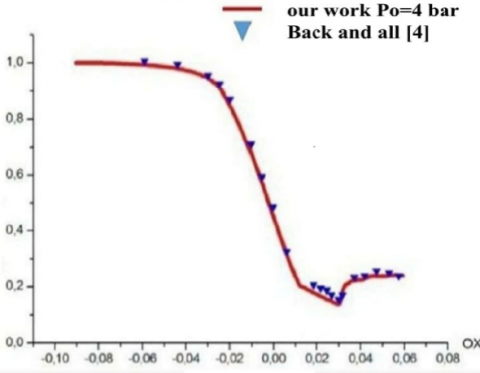
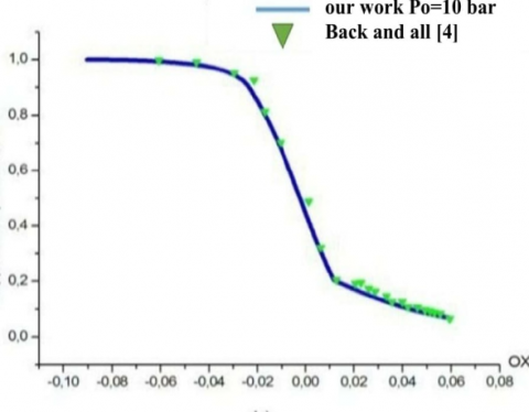
The present model is compared with the results due to Back and al. [4]. As shown in Figures 2a and 2b, static to stagnation pressure ratio is in good agreement between the two works.
Figur 2a. Ratio of the pressure comparison between our works And that of Back and al. [4]
Figure 2b. Ratio of the pressure comparison between our works and that of Back and al. [4]
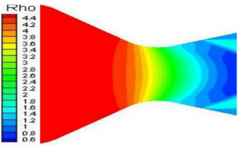
Figure 3. Contours of density (kg / m3) (Po=4 bar)
Figure 3 shows the density profile (color change) that takes two different paths; the first surface from the entrance of the nozzle to its neck, the density in this part is almost constant at its maximum value. The second surface that begins just after the neck of the nozzle, the density undergoes a small increase and then continues to decrease until the exit of the nozzle.
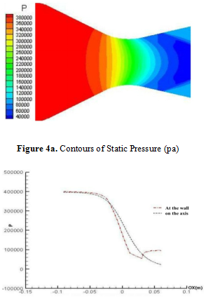
The pressure drop inside the nozzle is shown schematically in Figures 4a and 4b. qualitatively this profile follows almost the same form of density profile.
Figure 4b. Evolution of static pressure center and cell wall (Po=4 bar)
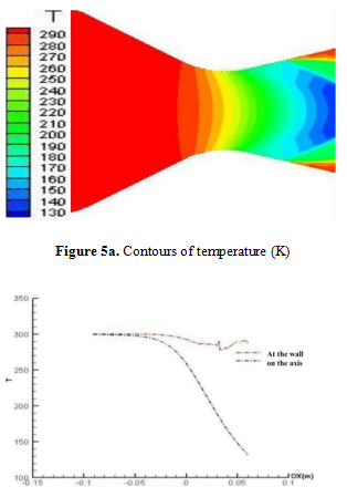
Figure 5b. Evolution of temperature center and cell wall (K) (Po=4 bar)
The temperature distribution and its evolution are shown respectively in Figs. 5a and 5b, the temperature in the middle of the nozzle is subject to a homogeneous and continuous descent until the exit.
The wall is slightly reduced with a small increase in different inputs before exiting the nozzle (shock wave), on the other hand the proportion of fixed wall distribution along the nozzle due to the friction between flow and walls.
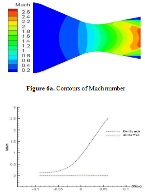
Figure 6b. Evolution of Mach number center and cell wall (Po=4 bar)
The evolution of the Mach number on the centre and the wall of the nozzle shown in Figures 6a and 6b respectively, we observe that the regime at the inlet of the nozzle remains almost constant or invariable up to axis of the nozzle. We can say that the regime is subsonic (Ma <1). We can neglect the air compressibility for Mach numbers less than 0.3, because the value of the Mach number is strictly less than unity, then there is a sharp increase in the vicinity of the neck of the nozzle exactly between the first point of tangency at the convergence and the first point of tangency in the divergent. In this zone the regime becomes transonic (0.94 <Ma <1.2), because there is a small decrease on the centre of the nozzle. At the entrance of the diverging zone, the value of Mach number inside the nozzle continues to increase until the exit of the nozzle in this zone, the regime is hypersonic (Ma> 5). The same observations for the evolution of the Mach number except in parietal disturbance in the vicinity of the neck due to friction between the fluid and the wall. The convergent-divergent profile of the nozzle accelerates the gas from subsonic speed to supersonic speed that causes the displacement.
This computational result examined the effects of several parameters on the dynamic and thermal characteristics of flow through a cooled convergent-divergent nozzle. The computational results indicated the following:
For an initial pressure, Po, inferior to the critical pressure, Pc, the delamination position is affected by this pressure difference and moves the nozzle throat. On the other hand, if the initial pressure is greater than the critical pressure, the release moves the lip of the nozzle until its disappearance which is desirable. Therefore, the delamination, which is an undesirable, phenomenon, appears in some flows, particularly when the initial pressure is below to the critical pressure. This could be causes the degradation of nozzle aerodynamic performances and efficiency and also causes noise and structure vibrations. So, in order to avoid these disadvantages, it is important to increase the initial pressure and make an optimal choice of the nozzle outlet angle.
|
$k$ |
turbulent kinetic energy |
|
$\omega$ |
specific turbulent dissipation rate |
|
$\mu$ |
dynamic viscosity |
|
t |
turbulent viscosity |
|
$p$ |
density |
|
$\Omega$ |
scalar measure of the vortices tensor |
|
$\Omega_{i j}$ |
vortices tensor |
|
$\gamma$ |
specific heat ratio |
|
$a_{1}$ |
brdshow constant |
|
$r$ |
radius, radial coordinate, recovery factor |
|
$\chi$ |
axial coordinate |
|
$T$ |
Temperature |
|
$M a$ |
Mach number |
|
$P$ |
Pressure |
|
$P r_{t}$ |
turbulent Prandtl number
|
|
$U_{i}$ $u_{i}$ |
mean velocities fluctuating velocities |
|
$h$ |
heat transfer coefficient |
|
$P r$ |
Prandtl number |
|
$e$ |
free stream condition |
|
$\mathrm{F} 1, \mathrm{F} 2$ |
auxiliary functions in turbulence model |
|
$t$ |
Time |
|
Subscripts |
|
|
0 |
nozzle entrance condition |
|
$t h$ |
throat position |
|
$S e p$ |
separation position |
|
$W$ |
parameters on the wall surface |
|
$a w$ |
adiabatic wall |
[1] Back L.H., Massier P.F., Gier H.L. (1964). Convective heat transfer in a convergent-divergent nozzle, Int. J. Heat Mass Transfer, Vol. 7, pp. 549-68.
[2] Lutum E., von Wolfersdorf J., Semmler K., Dittmar J., Weigand B. (2001). An experimental investigation of film cooling on a convex surface subjected to favourable pressure gradient flow, Int. J. Heat Mass Transfer, pp. 939-951.
[3] Lebedev V.P., Lemanov V.V., Terekhov V.I. (2006). Film-cooling efficiency in a Laval nozzle under conditions of high free stream turbulence, Journal of Heat Transfer, Vol. 128, pp. 571-579.
[4] Back L.H., Massier P.F., Gier H.L. (1965). Comparison of measured and predicted flows through conical supersonic nozzles, with emphasis on the transonic region, AIAA Journal, Vol. 3, No. 9, pp. 1606-1614.
[5] Cuffel R.F., Back L.H., Massier P.F. (1968). Transonic flow field in a supersonic nozzle with small throat radius of curvature, December, AIAA paper, Vol. 17, No. 7, pp. 1364-1366.
[6] Souici M. (2012). Étude d'un écoulement compressible dans uneTuyère convergente divergente, Laghouat university.
[7] Lorenzini G., Saro O. (2016). Analysis of water droplet evaporation through a theoretical numerical model, International Journal of Heat and Technology, Vol. 34, Spe. 2, pp. S189 - S198. DOI: 10.18280/ijht34S201
[8] Perrot Y. (2006). Etude mise au point et validation de modèles de turbulence compressible, Institut National des Sciences Appliquées de Rouen France.