OPEN ACCESS
The paper presents a numerical prediction of reacting flow field and temperature distribution of turbulent diffusion flame in two air blast nozzle swirling flow namely co and counter with different swirl intensities. This quantity is 0.46 for the central flow and ± 1.0 for the annular flow. Current study was focus on the rotation effect of the secondary flow. The calculated results were validated on real time through laser anemometry for both cases. The reasons behind the choice of this issue is that it is realistic in the industry but with a larger scale and our possession of the experimental values to validate the simulation. The use of two flows produced less NOx than a single flow due to its high capacity which homogenizes the temperature in the burner. The obtained results show that LES had successfully predicted the recirculation zones (CTRZ and CRZ) and the PVC with good precision.
swirl, large eddy simulation, turbulence, flame, co and counter swirl
Throughout the world, environmental agencies are currently requiring even lower rates of emissions of NOx and other pollutants from both new and existing gas turbines. Consequently, reducing pollutant emissions constitutes one of the most challenging areas in combustion research towards sustainable economic future, involving fuel consumption reduction and combustion efficiency.
Since one of the effective ways to reduce NOx emission is to decrease the flame temperature [1], a variety of pre-formation and post-formation control technologies have been employed, either individually or in combination. Among the former, lean premixed (LPM) combustion is the most promising to fulfill the regulatory requirements [2-5]. In LPM combustion systems, the air and fuel are thoroughly mixed upstream of the reaction zone to form a lean mixture. This excess air is a key to limiting NO formation, as very lean conditions cannot produce the high temperatures that produce thermal NOx. Unfortunately, this style of combustor is prone to serious problems related to combustion instabilities, flashback phenomena, instabilities or CO formation because of the very low temperature [6-11]. In addition, the design of a successful LPM combustor requires the development of hardware features and operational methods that simultaneously allow the equivalence ratio and residence time in the flame zone to be low enough to achieve low NOx emissions, but with acceptable levels of combustion dynamics, stability at part-load conditions and sufficient residence time for CO burnout [12].
As an alternative of LPM, non-premixed flames may provide a safer operation and avoid the above-mentioned undesirable combustion phenomena. Non-premixed flames are established when fuel and oxidizer are not mixed before they enter the combustion chamber. The mixing process of both components plays an important role in the combustion process, since the reactants species have to reach the reaction region.
To achieve this requirement the burner design is commonly based on the common injection of air and gaseous fuel in the form of swirling flow. It results in an enough adverse pressure along the axis, forming a swirl-induced central toroidal recirculation zone (CTRZ) which is only formed beyond a critical value of the swirl number, around 0.5~0.6 [13]. Once the CTRZ is established, it anchors the flame, thus improving the flame stabilization by returning hot gases and active radicals back to the jet core leading to a more stirred mixture. The shear layer between this recirculation zone and the main flow zone also generates great amount of turbulent energy, which intensifies the air-fuel mixing process and therefore improves the combustion efficiency, reduces the flame length, and lowers significantly the emission of NOx [14-19].
Most modern gas turbines use double-concentric swirl-burner because it gives the freedom to vary the distribution of axial and angular momentum of different airflow and mixing patterns can be achieved, resulting in substantial reduction in NOx emissions and lean blow off (LBO) limit in comparison to single swirler burner [20]. This technology is attractive to fit producing the required power in small size and compact combustor because several ignitions are distributed at the combustor head without any side wall among igniters. So, the more detail understanding of the dynamic flow and mixing in this annular combustor is very important to improve engine power and efficiency. Such reasons are closely related to the motivation of this study.
On the other hand, the fast development of computer and methodology of numerical computation technology have enabled computational fluid dynamics (CFD) to play a great role in designing combustors design because of its low cost compared with experimental testing. CFD is very effective when used as a guide for potential experimental investigations, particularly when experimental data is available for at least one test condition, for comparison with the CFD predictions.
Since the accuracy of mixing predictions for these flows plays a crucial role in the simulation of gas turbine combustion, a number of CFD studies were carried out to get information on the swirling flow field inside the combustor but prediction of such a flow pattern pose a daunting challenge since the developed recalculating flow pattern is the result of a multitude of complex processes involving strong shear regions, high turbulence, very large curvature of streamlines within the flow and rapid mixing rates.
In the number of recent studies, Large Eddy Simulation (LES) and Direct Numerical Simulation (DNS) were used to study the patterns of flow and mixing which occur in recalculating swirling flows. Such simulation strategies, while having the potential of becoming practical simulations tools with the rapid advances in computing power, are still prohibitively expensive for practical applications and remain somewhat impractical for routine engineering design which still relies on the solution of Reynolds-averaged equations with associated turbulence closures. The motivation of the present work has been to make a direct comparison between the results of calculations and experiments and to make the results of the calculation contribute to the improvement of the experimental methods.
In the present work the turbulence reacting gas and air in a turbine model combustor (GTMC) has been numerically simulated. The LES turbulence model was considered. To elaborate their strengths and weakness the simulation results were compared with the experimental data obtained by laser Doppler velocimetry [19]. The validation is comprised of the (time-averaged) profiles of flow velocities.
The balance equations governing the reacting flow are: mass, momentum, species and energy. The founder idea of large eddy simulation (LES) is to resolve the large turbulent motions in a flow field and to modeling only the effects of small ones. The resolved contribution $\overline{f}$ is obtained by applying the spatial LES filter to instantaneous variables f. Filtering the instantaneous governing equations and introducing the Favre filtered variables $\tilde{f}=\overline{f} \rho / \overline{\rho}$ [17-18].
$\frac{\partial \overline{\rho}}{\partial t}+\nabla \cdot\left(\overline{\rho} \tilde{u}_{i}\right)=0$ (1)
Motentum quantity conservation equation:
$\frac{\partial}{\partial t}\left(\overline{\rho} \tilde{u}_{i}\right)+\frac{\partial}{\partial x_{l}}\left(\overline{\rho} \tilde{u}_{i} \tilde{u}_{l}\right)=-\frac{\partial \overline{P}}{\partial x_{i}}+\frac{\partial}{\partial x_{l}}\left(\overline{\tau}_{i l}-\overline{\rho}\left(\widehat{u_{i}^{\prime} u_{l}^{\prime}}-\tilde{u}_{i} \tilde{u}_{l}\right)\right.$ (2)
Chimical species conservation equation:
$\frac{\partial}{\partial t}\left(\overline{\rho} \tilde{Y}_{k}\right)+\frac{\partial}{\partial x_{i}}\left(\overline{\rho} \tilde{u}_{i} \tilde{Y}_{k}\right)=\frac{\partial}{\partial x_{i}}\left(\rho \tilde{D}_{k} \frac{\partial \tilde{Y}_{k}}{\partial x_{i}}-\overline{\rho}\left(\overrightarrow{u_{i} Y_{k}}-\tilde{u}_{i} \tilde{Y}_{k}\right)\right)+\overline{\omega}_{k} ; \ldots \ldots k=1, N$ (3)
Energy conservation equation:
$\frac{\partial}{\partial t}\left(\overline{\rho} \tilde{h}_{s}\right)+\frac{\partial}{\partial x_{i}}\left(\overline{\rho} \tilde{u}_{i} \tilde{h}_{s k}\right)=\frac{\partial \overline{p}}{\partial t}+\tilde{u}_{i} \frac{\partial \overline{p}}{\partial x_{i}}+\frac{\partial}{\partial x_{i}}\left(\lambda \frac{\partial \tilde{T}}{\partial x_{i}}-\overline{\rho} \widetilde{\left(u_{i} h_{s}\right.}-\tilde{u}_{i} \tilde{h}_{s}\right)-\sum_{k=1}^{N} \dot{\dot{\omega}}_{k} \Delta h_{f, k}^{0}$ (4)
Gas state equation:
$\overline{P}=\overline{\rho} \tilde{r} \tilde{T}$ (5)
where: Ui and u’i are the components average and fluctuating velocity in the direction xi, Yk is the methane mass fraction, P is the pressure, μ is the dynamic viscosity and ρ is the density of the fluid. The hs is the sensible enthalpy, λ is the thermal conductivity; Dk is the species diffusivity; Is estimate to the ratio of kinematic viscosity to Schmidt number ScK which is assumed to be 0.7 in this study.; T is the temperature; $\dot{\omega}_{k}$ is the secrecies reaction rate and the $\Delta h_{f, k}^{0}$ is the formation enthalpies of species. Mass flux is described by Fick’s law in the equation (3).
The viscous heating term and radiation term in equation (4) are neglected as they are negligible compared to the combustion source term. $\overline{\tau}_{i l}$ is The stress tensor and the deviatoric part of filtered strain tensor is define us:
$\tilde{S}_{i j}=\left(\frac{1}{2}\right)\left(\left(\frac{\partial \tilde{u}_{i}}{\partial \tilde{x}_{j}}\right)+\left(\frac{\partial \tilde{u}_{j}}{\partial \tilde{x}_{i}}\right)\right)$ .
In this calculating method of turbulent flows offers a good compromise between computational cost and adequate description of unsteady turbulence.
The LES equations are obtained by filtering the Navier-Stokes equations at the scale l. In a calculation code LES, the filtering operation is carried out implicitly by the mesh and the numerical scheme: the structures of the turbulence smaller than l are not solved by the calculation but taken into account by the model LES. The dissipation and dispersion errors of the numerical scheme contribute to the increase of the filter size. For more detailed concerning LES approach, we refer to [24].
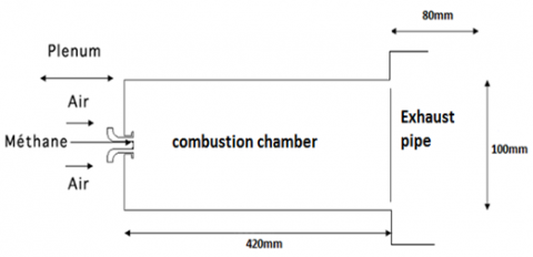
The Adopted configuration has been investigated experimentally [19], through laser Doppler anemometry (LDA). It consists of two co-swirling air flows injected through a central nozzle (diameter 15 mm) and an annular nozzle (i.d. 17 mm, o.d. 25 mm widening to 30 mm at the exit). Non swirling gaseous fuel (CH4) is injected through an annular slit between both airflows which results in a high degree of premixing before ignition at a few millimeters upstream the burner exit.
The diameter of the combustion chamber is DCC=4D0 and its length is DCL=18D0. Limitation of the main reaction zone was provided by an orifice with 70% diameter reduction placed at the exit of the combustion chamber. This outlet geometry avoids back-flow through the exit section, otherwise could be induced by the lowered pressure on the axis of the rotating fluid. The flow is axially accelerated by the constriction at the outlet of the combustion chamber. This helps to turn the flow from a subcritical state after the vortex breakdown to a supercritical flow at the outlet [4]. Based on these measurements, the sensitivity of the recirculation region to the outlet conditions can be reduced.
The mass flow rates of air and methane were adjusted at $\dot{M}_{a}$ =64kg/h and $\dot{M}_{f}$ =1.8kg/h, corresponding to an air equivalence ratio λ=2 and a through-flow time of 180ms $Y_{f, 0}=0.02735562$ . The air stream through the nozzle was electrically preheated up to 400°C (ρ=1.0924kg/m3μ=1.95710-5kg/s-m) and split between the inner circular passage (0.37 $\dot{M}_{a}$ ,23.68kg/h, 35.80m/s,Rei=962) and the outer annular canal. The global Reynolds number is calculated as the product of the axial average air velocity (U0=34.83m/s) at the nozzle exit defined as z=0 and the throat diameter of the diffuser divided by the kinematic viscosity of air and gives approximately
The swirl strength is characterized by the outlet swirl number S0, defined as the ratio of angular to axial momentum flux in the nozzle divided by the outside nozzle radius R0 as given by:
$S_{0}=\frac{\int_{0}^{R_{0}} \rho\left(\overline{U} \overline{W} r+\overline{u^{\prime} w^{\prime}} r\right) r d r}{R_{0} \int_{0}^{R_{0}} \rho\left(\overline{U}^{2}+\overline{u^{\prime}}^{2}\right) r d r}$ (6)
Figure 1. Geometrical configuration
The theoretical swirl number Sth calculated from only the geometrical data of the swirl generator is used since it is approximately equal to S0 [21]. It is of the inner airflow Sth,in=0.46 and of the outer air flow Sth,out=1.0, yielding the overall swirl number is Sth,total=0.81. This geometrical configuration is shown on Fig. 1, For more detailed specifications concerning the combustor, we refer to [19].
One of the crucial steps to modeling combustion in ansys fluent 14.0 is the choice of combustion model. So we must first choose a Premixed Combustion or Non-Premixed Combustion options. This determines whether or not the reactants present are initially mixed. From this stage, several choices of combustion model are available to us. Here we want to study a turbulent diffusion flame (Non-Premixed Combustion). In this model, it need to create the PDF table, where all parameters and its information’s on thermo-chemistry interactions with turbulence are adopted. All quantities values or all species like as fuel and oxide at the inlet has been induced in their experimental values cited in fourth parts and controlled in the PDF table. The PDF table over view to display temperature and reacting species: methane, oxygen and carbon dioxide with mixture fraction Figure 2 below. We can see that the maximum of temperature is 2200K corresponding to 0.125 of mixture fraction.
Figure 2. Temperature and different species evolution with mixture fraction
In this investigation; ANSYS-Fluent 14.0 CFD software has been used in which was intensely validated and compared well with the experience. The solver is based on the finite volume method for resolving all transport equations. Turbulence was modeled by the LES (large eddy simulation) with the WALE subgrid-scale viscosity has been considered. The default scheme time discretisation assumed in this study was the second order. PISO, algorithm procedure was used for coupling the pressure and velocity fields for incompressible flow. By using this solver; the equations show a fast convergence. All equations are resolved numerically in unsteady case using a grid of 0.80 million hexahedral cells with convergence criteria about 10-6. Three types of boundary conditions were applied in this study; Inlet, outlet and wall. At the input of the combustion chamber all values of different parameters are measurements; like the velocities (U, V, W) species and turbulent kinetic energy by a specifically UDF algorithm of profiles type [26-28]. Except dissipation of turbulent kinetic energy which is calculated by this equation:
$\varepsilon=C_{\mu}^{0.75} \frac{k^{1.5}}{0.7 D}$ (7)
where this value (0.7), was chosen after calculation and optimized with different test.
An outflow boundary condition was imposed at the exhaust.
Adiabatic walls were used for all combustion chamber. At axial axis of the combustion chamber we were define different abscissa (axial positions) from: x=2.5mm to x=150mm, Corroborates with the measuring points [19]. We can plot all radial parameters profiles from these positions.
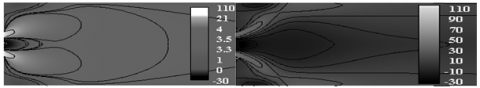
Figures 3, 4 and 5 shows the fields of the mean velocity components in the combustion chamber. By preserving the flow flux, the jet is very strongly accelerated in the diffuser of the injector. The tangential component, Figure 5 recalls that the flow is very strongly swirled. The jet then opens into the chamber where it opens in two steps, as can be seen in Figure 4 for the two cases co and counter swirl. In fact, the bursting due to the swirl is initially limited by the straight diffuser which confines the jet. On the axial component, Figure 3, this phenomenon can be observed. The central recirculation zone has the shape of a bottle neck (in the literature) and has two toroidal cells. The presence of the recirculation zones in the corners (for z<30 mm) is shown in Figures 3 and 5, which can no longer be seen in after. Far from the walls, the flow is axisymmetric; Never the less, axisymmetry is Broken. At the outlet of the injector, the shear is very important because the very fast jet lies between the central zone and the corner zones. At the outlet of the injector, the shear is very important because the very fast jet lies between the central zone and the corner zones. It will be seen that these places are conducive to the appearance of strong hydrodynamic instabilities.
Figure 3. Contours of axial velocities: left co swirl; right counter swirl
Figure 4. Contours of radial velocities: left co swirl; right counter swirl
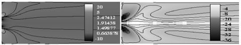
Figure 5. Contours of tangential velocities: left co swirl; right counter
Before proceeding further, it is important to ensure the reliability and accuracy of the Current code of LES. To this end, a comparison of the predicted results and the experimental data is made for the axial, radial and tangential velocities. The expected results are generally in good agreement with the experimental data. In particular, the position of the maximum speed is reproduced well by numerical calculation. In addition, the agreement is satisfactory for the recycling region. Validation of the model is also evaluated with comparison to the experimental data.
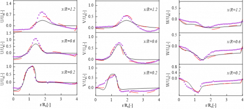
Quantitative comparison between obtained results and experimental data provided by [19] has been presented, in three different sections: 2.5mm, 7.0mm and 15mm for two cases. Traces Profiles are given in Fig.6, as well as indicated the presence of the recirculation zones. These profiles confirm the qualitative observations, such as the presence of a bottle-shaped of central toroidal recirculation zone (CTRZ) and corner recirculation zone (CRZ). Moreover, the curves are symmetrical with respect to the main axis, in the zone near to the injector, which is no longer true downstream. The obtained results are very satisfactory, the agreement between calculations and experiments still good for all velocity averages of components, in particular for the axial velocity and at entire abscissas of comparison. Position of the recirculation zones, as well as the opening of the jet, is very well predicted. The speed levels, especially near the injector area, are well reflected in the simulation, except for small overestimation of the negative velocity zone at the center of the CTRZ on the third profile. These data allow a posteriori to validate the method used to solve Flow in this proposed configuration.
Figure 6. Profiles of axial; radial and tangential velocities in two cases co and counter swirl
OOO Exp. –––– Co swirl. – – – Counter swirl
The contours of the vorticity for two cases are illustrated in the Figure 7. This parameter designs the measure rotation rate of particle flow; it can also give information on the horizontal shear (this is why we can identify the fronts by looking at the vertical vorticity).
The shown dynamic of the fluid is mainly its rotational movement about the axis, so the type of flow is swirled for both cases with a different direction of rotation according to our consideration.
Figure 7. Contours of vorticity: left co swirl; right counter swirl
Figure 8 mainly shows the presence of instabilities, thanks to Q criterion is surfaces. This makes it possible to detect vortex structures or PVCs with pressure is surfaces, because this is the zone of lowest pressure in the configuration, with comparison between tensor of deformations SIJ and tensor of rotational speeds these instabilities are PVC: Processing vortex cores wind around the CTRZ or the Vortex rings: Kelvin Helmholtz instabilities are formed at the level of the shear layer located at the border between the CRZ and the jet. These create ring eddies. Parameters influencing these phenomena; is the tangential movement in axisymmetric flows induces centrifugal forces, which are balanced by a radial gradient of static pressure:
$\frac{W^{2}}{r}=\frac{1}{\rho} \frac{\partial p}{\partial r}$ (8)
Thus generates a minimum of pressure at the symmetric axis and positive gradient towards the jet boundary [19].
Figure 8. Contours of Q: left co swirl; right counter swirl
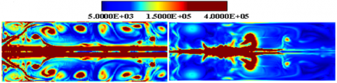
In the Figure 9 we show the mean field contours of the temperature in the two cases. It’s uniform and equal to the command value at the inlet expansion section. Just downstream of expansion, temperature begins to rise sharply, indicating the start of combustion. Isothermal contours clearly illustrate the shape of the flame front. The maximum temperature “1800 K” is reached on the axis at central recirculation zone. The combustion is almost complete with x = 0.20 m and there is no longer fresh gas beyond this section (on average). Note that, we do not observe thermal boundary layers along the combustion chamber walls because supposed adiabatic. As can be seen from Fig.9, the difference between co and counter swirl is only in the corner zone. Thus the heat flux loss through the combustion chamber walls at this section about 7% between the direct and counter-direction or the region of jet dominated on itself, thus two diameters of inlet nozzle of combustion chamber [19]. As comparison, the maximum temperatures significantly lower as low as 1850° K can be seen in the co swirl assembly. In summary of this interpretation we can saw that the Methane is injected directly into the chamber; flame is not attached at the injector lips because the flow velocity is too great. The rich zones are delimited by the stoichiometric line, inside this; a rich premix pocket is formed, while on the outside, the premix is poor.
The rich zone burns in premix (corresponding to the pink contours of the reaction rate in Figure 9). Behind the front flame, air coming from the inner twirling flow (central swirler) is heated by the burnt gases retained in the central recirculation zone. This diluted air will burn in diffusion with the excess fuel coming from the rich premix flame. The burned gases returned to the recirculation zone of the step, warm the fresh mixture. On the whole, it can be seen that the areas where the flame burns in diffusion are very minor as in compared with burns zone flame in premix.
The average fields reveal that the flame is compact and stabilized near the injectors for both cases co and counter swirl.
Figure 9. Contours of temperature: left co swirl; right counter swirl
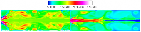
The temperature fluctuations and kinetic energy are identical Fig 10. Remains to say that the peaks of energy in the counter case are greater than that of the co swirl at immediate line. The stability criteria of Rayleigh explain these phenomena [20-22].
Figure 10. Contours of kinetic energy: left co swirl; right counter swirl
6.1. Spectral analysis
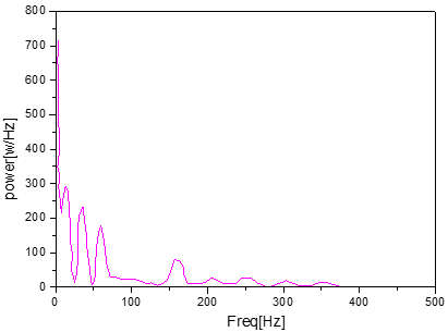
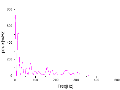
Figures 11 and 12 shows the power spectrum of the time signal for pressure at the considered point at x = 10.5 mm y=1.5mm in axial and radial direction for both cases co and counter swirl. This power spectrum was obtined by applying the Fast Fourier Transform (FFT) for statistics instantaneous pressure. Interest mainly in the energy components of the spectral amplitude density of, the Strouhal number corresponding to the periodic phenomena is:
$S_{t}=\frac{f d_{\mathrm{in}}}{u_{i n}}$ (9)
Or uin is the velocity at the outlet of the injector, din is the exit diameter of the diffuser and f the PVC frequency. In our study; din = 50mm and the power spectrum for the co swirl has a distinct peak at a frequency of f = 26Hz and 34Hz for counter swirl. when the uin equal to 34.82m/s for both cases.
An author definition given by [20] after an experimental study or the Strouhal number is given by
$S_{t}=\frac{2 f r_{\mathrm{in}}}{W_{i n}}$ (10)
Or; f is the PVC frequency, rin is the diffuser radius and Win is the tangential velocity at inlet of the diffuser.
Strouhal number corresponding to the both cases co and counter swirl is 0.18 and 0.25 respectively.
Figure 11. Power spectrum for Co swirl
6.2 Combustion and product species evolution
Figure 12. Power spectrum for counter swirl
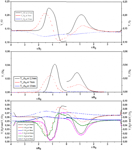
Figure 13. Profiles of different parameters at different sections of both cases left co swirl; right counter swirl
The methane mass fraction is represented by radial profiles at different positions, 2.5, 7 and 15 mm shown in Figure 13. The consumption of the fuel is clearly illustrated, because the mass fraction decreases from the initial value at the outlet of the jet and totally burned just in front of the flame to give dioxide carbon and water vapor. It has been observed that the excess of air is translated by an amount of oxygen which remains in the products of the combustion (rate of reaction). Among the species produced; the mass fraction of CO2 is also expressed as radial profiles in last positions. The behavior of H2O is similar to CO2. By crossing the front flame the mass fraction is increased to reach maximum values. Downstream of the front flame, the concentration of these species decreases since they mix with the air of the surrounding [23]. The intermediate specie CO as defined in the reduced reaction mechanism at two stapeses of Peters and Williams is illustrated in Figure 12 where radial profiles are shown at also sections. The mass fraction of this component is zero in the burned gases and it maximum in the flame front, hence it’s characteristic of intermediate species: when the fresh gases cross the flame front, there is first a production of the species CO followed immediately it’s consumption to give CO2 and H2O. Finally, we can see that the profiles are similar in the two cases co and counter swirl.
In this paper, numerical results of turbulent diffusion flame were reported using the LES approach. This study is based on the experimental work of Merkel and all [19], where two geometrical configurations are considered with a change in rotation direction of the external fluid. The proceedings are divided into four parts; the friability of the model by comparing the numerical results and the experimentation. The second point is the detection of the flow structures in both cases co and counter swirl or it is proved that the second is strongly swirl with a higher recirculation rate regarding the quantity of mass reversed compared to co swirl. This point is well predicted in our previous studies Lalmi et al. [24] comparatively with Merkle and all [19].
The temperature evolution is well treated in the third parts of this paper or it has been proved that the fluctuations of temperatures are identical to the kinetic energy.
The centrifugal forces and the depression in the second case show that the kinetic energies are at greater peaks than the first case; these remarks were explained with the decay of the angular moment.
The last point is the spectral analysis power of the statistic pressure was confronted for predicted the processing vortex corps. After applying Fourier transform for static pressure, the spectral evolution shows that there is a very energetic range in two cases co and counter swirl. For Closing this parts the number of Strouhal calculation gives a general overview on the procession and the formation of procession vortex cops (PVC) at the end one can say that this work is completed their objective or model LES Capable of predicting vortex phenomena with complex geometries such as the second configuration (counter swirl) considered.
|
Yf |
Methane mass fraction |
|
Dcc |
Diameter of the combustion chamber( $D C C=4 D_{0}$ ) |
|
St |
Strouhal Number |
|
$f$ |
frequency |
|
D0 |
Diameter of central nozzle, m |
|
U0 |
Axial average air velocity |
|
Dcl |
length of combustion chamber ( $D_{C L}=18 D_{0}$ ), m |
|
Ma |
Air mass flow of, kg/h |
|
Mf |
Methane mass flow of kg/h |
|
Re |
Reynolds number |
|
Sth,in |
Theoretical Inner Swirling Number |
|
Sth,ex |
Theoretical outer swirling Number |
|
P |
Pressure, Pas |
|
K |
Turbulent Kinetic energy |
|
U |
Axial velocity, m/s |
|
V |
Radial velocity, m/s |
|
W |
Tangential velocity |
|
Greek Symbols |
|
|
ɛ |
Dissipation rate |
|
ʋ |
Kinematic viscosity |
|
ω |
Turbulent frequency |
|
$\lambda$ |
Air equivalence ratio |
[1] Billiant P., Chomaz J.M., Heurre P. (1998). Experimental study of vortex breakdown in swirling jets, J. Fluid Mech., Vol. 376, p. 183. DOI: 10.1017/S0022112098002870
[2] Valera-Medina A., Syred N., Griffiths A. (2009). Visualization of isothermal large coherent structures in a swirl burner, Comb. Flame, Vol. 156, pp .1723-1734.
[3] Chen R.H., Driscoll J.F. (1988). The role of the recirculation vortex in improving fuel-air mixing within swirling flows, Proc. Combust. Inst., Vol. 22, p. 531.
[4] Escudier M. (1988). Vortex breakdown: Observations and explanations, Prog. Aero. Sci., Vol. 25, pp. 189-229. DOI: 10.1016/0376-0421(88)90007-3
[5] Lucca-Negro O., O’Doherty T.O. (2001). Vortex breakdown: A review, Prog. Ener. Comb. Sci., Vol. 27, pp. 431-481. DOI: 10.1016/S0360-1285(00)00022-8
[6] Pierce C.D., Moin P. (1998). Method for generating equilibrium swirling inflow conditions, AIAA J., Vol. 36, pp. 1325-1327. DOI: 10.2514/2.518
[7] Wegner B., Maltsev A., Schneider C., Sadiki A., Dreizler A., Janicka J. (2004). assessment of unsteady RANS in predicting swirl flow instability based on LES and experiments, Int. J. Heat and Fluid Flow, Vol. 25, pp. 528-536. DOI: 10.1016/j.ijheatfluidflow.2004.02.019
[8] Wegner B., Kempf A., Schneider C., Sadiki A., Dreizler A., Janicka J., Schäfer M. (2004). Large eddy simulation of combustion processes under gas turbine conditions, Prog. Computational Fluid Dynamics, Vol. 4, pp. 257-263. DOI: 10.1504/PCFD.2004.004094
[9] Chenzhou L., Charles L., Merkle (2011). Contrast between steady and time-averaged unsteady combustion simulations, Computers & Fluids, Vol. 44, pp. 328-338.
[10] Dinesh K.R., Kirkpatrick M.P. (2009). Study of jet precession, recirculation and vortex breakdown in turbulent swirling jets using LES, Computers & Fluids, Vol. 38, No. 6, pp. 1232-1242.
[11] Syred D.G., Beer J. (1974). Combustion in swirling flows: A review, Comb. Flame, Vol. 23-2, pp. 271-305. DOI: 10.1016/0010-2180(74)90057-1
[12] Fröhlich J., Garcia V.M., Rodi W. (2008). Scalar mixing and large-scale coherent structures in a turbulent swirling jet, Flow, Turbulence and Combustion, Vol. 80, No. 1, pp. 47-59.
[13] Roux S., Lartigue G., Poinsot T., Meier U., Berat C. (2005). Studies of mean and unsteady flow in s a swirled combustor using experiments, acoustic analysis and large eddy simulations, Combust. Flame, Vol. 141, pp. 40-54. DOI: 10.1016/j.combustflame.2004.12.007
[14] Malalasekera W., Ranga K.K.J., Dinesh S.S., Ibrahim M.P., Kirkpatrick (2007). Large eddy simulation of isothermal turbulent swirling jets, Combust. Sci. and Tech., Vol. 1791, pp. 481-1525. DOI: 10.1080/00102200701196472
[15] Hadef R., Lenze B. (2008). Effects of co- and counter swirl on the droplets characteristics in the spray flame, Chemical Eng. Process Intensification, Vol. 47-12, pp. 2209-2217. DOI: 10.1016/j.cep.2007.11.017
[16] Syred N., Beer J.M. (1974). Combustion in swirling flows: A review, Combustion and Flame, Vol. 23, No. 2, pp. 143-201. DOI: 10.1016/0010-2180(74)90057-1
[17] Pierce C.D., Moin P. (1998). Large eddy simulation of a confined coaxial jet with swirl and heat release, AIAA Paper, p. 2892. DOI: 10.1016/0010-2180(74)90057-1
[18] Pierce C.D., Moin P. (1998). Method for generating equilibrium swirling inflow conditions, AIAA J., Vol. 36, No. 7, pp. 1325-1327. DOI: 10.2514/3.13970
[19] Merkle K., Haessler H., Büchner H., Zarzalis N. (2003). Effect of co- and counter-swirl on the isothermal flow-and mixture-field of an airblast atomizer nozzle, International Journal of Heat and Fluid Flow, Vol. 24, No. 4, pp. 529-537. DOI: 10.1016/S0142-727X(03)00047-X
[20] Nicolaus D.A., Smith C.E. (2005). Analysis of highly swirled, turbulent flows in dump combustor with exit contraction, ASME Paper GT2005-68160. DOI: 10.1115/GT2005-68160
[21] McIlwain S., Pollard A. (2002). Large eddy simulation of the effects of mild swirl on the near field of a round free jet, Physics of Fluids, Vol. 14, No. 2, pp. 653-661. DOI: 10.1063/1.1430734
[22] Kumar R., Sood S., Sheikholeslami M., Shehzad S.A. (2017). Nonlinear thermal radiation and cubic autocatalysis chemical reaction effects on the flow of stretched nanofluid under rotational oscillations, Journal of Colloid and Interface Science. DOI: 10.1016/j.jcis.2017.05.083
[23] Kumar R., Sood S. (2017). Combined influence of fluctuations in the temperature and stretching velocity of the sheet on MHD flow of Cu-water nanofluid through rotating porous medium with cubic auto-catalysis chemical reaction, Journal of Molecular Liquids, Vol. 237, pp. 347-360. DOI: 10.1016/j.molliq.2017.04.054
[24] Zhiyin Y. (2015). Large-eddy simulation: Past, present and the future, Chinese Journal of Aeronautics, Vol. 28, No. 1, pp. 11-24. DOI: 10.1016/j.cja.2014.12.007
[25] Lalmi D., Hadef R. (2015). Numerical simulation of co and counter swirls on the isothermal flow and mixture field in a combustion chamber, Advances and Applications in Fluid Mechanics, Vol. 18, No. 2, pp. 199-212. DOI: 10.17654/AAFMOct2015_199_212
[26] Triveni M.K., Panua R. (2017). Numerical analysis of natural convection in a triangular cavity with different configurations of hot wall, International Journal of Heat and Technology, Vol. 35, No. 1, pp. 11-18. DOI: 10.18280/ijht.350102
[27] Mansouri Z., Mokhtar A., Boushaki T. (2016). A numerical study of swirl effects on the flow and flame dynamics in a lean premixed combustor, International Journal of Heat and Technology, Vol. 34, No. 2, pp. 227-235. DOI: 10.18280/ijht.340211
[28] Ambethkar V., Kushawaha D. (2017). Numerical simulations of fluid flow and heat transfer in a four-sided lid-driven rectangular domain, International Journal of Heat and Technology, Vol. 35, No. 2. DOI: 10.18280/ijht.350207