Influence of Hall and ion-slip currents on unsteady MHD free convective flow of a rotating fluid past an oscillating vertical plate

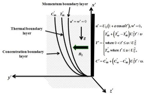
In Cartesian coordinate system $\left( {x}',{y}',{z}' \right)$, consider the unsteady MHD flow of an incompressible, chemically reacting, electrically and thermally conducting fluid past an infinite vertical plate ($-\infty \le {x}'\le \infty ,\,\,-\infty \le {z}'\le \infty $) embedded in a fluid saturated porous medium. The  ${x}'$-axis and ${z}'$-axis are in the plane of the plate and  ${y}'$-axis is normal to it. The flow past vertical plate is permeated by a uniform transverse magnetic field  ${{B}_{0}}$ which is parallel to  ${y}'$-axis and the whole flow system is in rigid body rotation with a uniform angular velocity  $\overrightarrow{\Omega }$ about  ${y}'$-axis. Initially, when time  ${t}'\le 0,$ the plate and the fluid are at rest. The plate temperature is assumed to be  ${{{T}'}_{\infty }}$ and species concentration at the surface of the plate and within the fluid is assumed to be... At time ${t}'>0$, the plate starts executing non-torsional oscillations in its own plane with a velocity  ${{U}_{0}}(1+\varepsilon \cos {\omega }'{t}')$ in  ${x}'$-direction. The plate temperature is increased linearly with time  ${t}'$ to  ${{{T}'}_{\infty }}+\left( {{{{T}'}}_{w}}-{{{{T}'}}_{\infty }} \right)U_{0}^{2}{t}'/\upsilon $ when  $0<{t}'\le \upsilon /U_{0}^{2}$ and thereafter it is kept at constant temperature  ${{{T}'}_{w}}$ when ${t}'>\upsilon /U_{0}^{2}$. At the same time, the species concentration at the surface of the plate is increased linearly with time  ${t}'$ to  ${{{C}'}_{\infty }}+\left( {{{{C}'}}_{w}}-{{{{C}'}}_{\infty }} \right)U_{0}^{2}{t}'/\upsilon $ and is kept same thereafter. The schematic diagram of the physical problem is shown in the Figure (1).

1.jpg

Figure 1. Schematic diagram of the physical problem

Since plate is infinitely extended along ${x}'$ and ${z}'$ directions so all physical variables shall be depend on  ${y}'$ and ${t}'$ only. In compatibility with the continuity equation the fluid velocity ${\vec{q}}'=({u}',\,{v}',\,{w}')$ may assume as ${\vec{q}}'=({u}',\,0,\,{w}')$. For metallic liquids and partially ionized fluids, magnetic Reynolds number ${{R}_{m}}={{U}_{0}}h/{{\eta }_{m}}\ll 1$ i.e. magnetic diffusivity is very large. This indicates that the induced magnetic field produced by fluid motion leaks through the conducting fluid point to point and so it is negligible in comparison to applied magnetic field (Cowling [30]). In essence of this assumption and solenoidal relation ($div{\vec{B}}'=0$) magnetic field ${\vec{B}}'=({{{B}'}_{x}},\,{{{B}'}_{y}},\,{{{B}'}_{z}})$ may assume as ${\vec{B}}'=(0,\,{{B}_{0}},\,0)$. Also, there is no addition/extraction of energy in the fluid in the form of electric field so the electric field ${\vec{E}}'=({{{E}'}_{x}},\,{{{E}'}_{y}},\,{{{E}'}_{z}})$ may assume as ${\vec{E}}'=(0,\,0,\,0)$ (Meyer [31]).

The general equation of motion for MHD free convective flow of an incompressible, chemically reacting, electrically and thermally conducting fluid past a vertical plate embedded in a porous medium in a rotating system is given by

 $\begin{align}  & \frac{\partial {\vec{q}}'}{\partial {t}'}+2\vec{\Omega }\times {\vec{q}}'=\upsilon {{\nabla }^{2}}{\vec{q}}'+\frac{1}{\rho }({\vec{J}}'\times {\vec{B}}')+\vec{g}{{\beta }_{T}}\left( {T}'-{{{{T}'}}_{\infty }} \right) \\ & +\vec{g}{{\beta }_{C}}\left( {C}'-{{{{C}'}}_{\infty }} \right)-\frac{\upsilon {\vec{q}}'}{{{k}'}}. \\\end{align}$      (1)

The energy equation with thermal diffusion is represented as

 $\frac{\partial {T}'}{\partial {t}'}=\frac{k}{\rho {{C}_{p}}}\frac{{{\partial }^{2}}{T}'}{\partial {{{{y}'}}^{2}}}-\frac{{{Q}_{0}}({T}'-{{{{T}'}}_{\infty }})}{\rho {{C}_{p}}}.$      (2)

The concentration equation with chemical molecular diffusion is given by

$\frac{\partial {C}'}{\partial {t}'}=D\frac{{{\partial }^{2}}{C}'}{\partial {{{{y}'}}^{2}}}-{K}'\left( {C}'-{{{{C}'}}_{\infty }} \right).$      (3)

Ohm’s law for a moving conductor taking Hall and ion-slip currents into account, is represented as (Sutton and Sherman [32])

  $\begin{align}  & {\vec{J}}'=\sigma \left[ {\vec{E}}'+\left( {\vec{q}}'\times {\vec{B}}' \right) \right]-\frac{{{\beta }_{e}}}{{{B}_{0}}}\left( {\vec{J}}'\times {\vec{B}}' \right) \\ & +\frac{{{\beta }_{e}}{{\beta }_{i}}}{{{B}_{0}}^{2}}\left( {\vec{J}}'\times {\vec{B}}' \right)\times {\vec{B}}'. \\\end{align}$    (4)

Using Eq (4) in Eq (1), the equation of motion for MHD free convective flow of an incompressible, chemically reacting, electrically and thermally conducting fluid past a vertical plate embedded in a porous medium in a rotating system taking Hall and ion-slip currents into account, in component form, become

 $\begin{align}  & \frac{\partial {u}'}{\partial {t}'}+2\Omega {w}'=\upsilon \frac{{{\partial }^{2}}{u}'}{\partial {{{{y}'}}^{2}}}-\frac{\sigma B_{0}^{2}}{\rho }\frac{\left( {u}'{{\alpha }_{e}}+{w}'{{\beta }_{e}} \right)}{\left( {{\alpha }_{e}}^{2}+{{\beta }_{e}}^{2} \right)} \\ & +g{{\beta }_{T}}\left( {T}'-{{{{T}'}}_{\infty }} \right)+g{{\beta }_{C}}\left( {C}'-{{{{C}'}}_{\infty }} \right)-\frac{\upsilon {u}'}{{{k}'}}, \\\end{align}$      (5)

$\frac{\partial w^{\prime}}{\partial t^{\prime}}-2 \Omega u^{\prime}=v \frac{\partial^{2} w^{\prime}}{\partial y^{\prime 2}}+\frac{\sigma B_{0}^{2}}{\rho} \frac{\left(u^{\prime} \beta_{e}-w^{\prime} \alpha_{e}\right)}{\left(\alpha_{e}^{2}+\beta_{e}^{2}\right)}-\frac{v w^{\prime}}{k^{\prime}}$    (6)

where  ${{\alpha }_{e}}=1+{{\beta }_{e}}{{\beta }_{i}}$.

The initial and boundary conditions specified for the present problem are given by

${t}'\le 0:\,{T}'={{{T}'}_{\infty }},\,\,{C}'={{{C}'}_{\infty }},\,\,\,{u}'={w}'=0\,\,\,\,\,\,\forall {y}',$         (7)

$\begin{array}{l}t' > 0:\\T' = \\\left\{ \begin{array}{l}{{T'}_\infty } + ({{T'}_w} - {{T'}_\infty })U_0^2t'/\upsilon \,\,{\rm{when}}\,\,\,0 < t' \le \upsilon /U_0^2,\\{{T'}_w}\,\,\,{\rm{when}}\,\,\,t' > \upsilon /U_0^2,\,\end{array} \right.\\C' = {{C'}_\infty } + \left( {{{C'}_w} - {{C'}_\infty }} \right)U_0^2t'\,/\upsilon ,\\u = {U_0}(1 + \varepsilon \cos \omega 't'),\,\,w' = 0\,\,\,{\rm{at}}\,\,\,y = 0,\\T' \to {{T'}_\infty },\,\,\,C' \to {{C'}_\infty },\,\,\,u' \to 0,\,\,w' \to 0\,\,\,as\,\,\,y' \to \infty\end{array}$       (8)

We now define the following non-dimensional quantities:

$\left. \begin{align} & y={y}'{{U}_{0}}/\upsilon ,\,\,u={u}'/{{U}_{0}},\,\,w={w}'/{{U}_{0}},\,\,t={t}'U_{0}^{2}/\upsilon , \\ & n={\omega }'\upsilon /U_{0}^{2},\,\,\,\theta =({T}'-{{{{T}'}}_{\infty }})/({{{{T}'}}_{w}}-{{{{T}'}}_{\infty }}),\,\, \\ & C=({C}'-{{{{C}'}}_{\infty }})/({{{{C}'}}_{w}}-{{{{C}'}}_{\infty }}). \\\end{align} \right\}$

Using above defined non-dimensional quantities and  $q=u+iw$ in Eqs (2-3) and (5-6), the Eqs (2-3) and (5-6) assume the following non-dimensional form

$\frac{\partial \theta}{\partial t}=\frac{1}{P_{r}} \frac{\partial^{2} \theta}{\partial y^{2}}-\phi \theta$        (9)

$\frac{\partial C}{\partial t}=\frac{1}{S_{c}} \frac{\partial^{2} C}{\partial y^{2}}-K_{1} C$     (10)

$\frac{\partial q}{\partial t}-2 i K^{2} q=\frac{\partial^{2} q}{\partial y^{2}}-M^{2}\left[\frac{\left(\alpha_{e}-i \beta_{e}\right)}{\left(\alpha_{e}^{2}+\beta_{e}^{2}\right)}\right] q+G_{T} \theta+G_{C} C-\frac{q}{k_{1}}$        (11)

where

The initial conditions (7) and the boundary conditions (8), in non-dimensional form, become

 $t\le 0:\,\,\,\theta =0,\,\,\,C=0,\,\,\,q=0\,\,\,\forall \,y$.      (12)

$\begin{array}{l}t > 0:\\\theta  = \\\left\{ \begin{array}{l}t\,\,\,{\rm{when}}\,\,\,0 < t \le 1,\\1\,\,\,{\rm{when}}\,\,\,t > 1,\end{array} \right.\\C = t,\,\,\,q = (1 + \varepsilon \cos nt)\,\,\,{\rm{at}}\,\,\,y = 0,\\\theta  \to 0,\,\,\,C \to 0\,,\,\,\,q \to 0\,\,\,\,\,{\rm{as}}\,\,\,y \to \infty\end{array}$         (13)

The mathematical model of the physical problem is presented by the coupled partial differential Eqs (9) to (11) together with the initial conditions (12) and boundary conditions (13).

The non-dimensional skin friction components at the plate in the primary flow direction ${{\tau }_{x}}$ and secondary flow direction ${{\tau }_{z}}$, for non-unit Prandtl and Schmidt numbers, are given by

Case (i) when  $n\ne {{X}_{2}}$

 $\begin{align}  & {{\tau }_{x}}+i{{\tau }_{z}}={{F}_{3}}\left( t,1,{{P}_{1}} \right)+\frac{\varepsilon }{2}\left[ {{e}^{\operatorname{int}}}{{F}_{3}}\left( t,1,{{P}_{2}} \right) \right. \\ & \left. +{{e}^{-\operatorname{int}}}{{F}_{3}}\left( t,1,{{P}_{3}} \right) \right]-\frac{{{G}_{T}}}{\left( {{P}_{r}}-1 \right){{A}^{2}}}\left[ {{F}_{3}}\left( t,1,{{P}_{1}} \right) \right. \\ & -{{F}_{3}}\left( t,{{P}_{r}},\phi  \right)+A\left( {{F}_{4}}\left( t,{{P}_{r}},\phi  \right) \right.\left. -{{F}_{4}}\left( t,1,{{P}_{1}} \right) \right) \\ & -{{e}^{-At}}\left( {{F}_{3}}\left( t,1,{{P}_{4}} \right)-{{F}_{3}}\left( t,{{P}_{r}},{{P}_{5}} \right) \right) \\ & -H(t-1)\left\{ {{F}_{3}}\left( t-1,1,{{P}_{1}} \right)-{{F}_{3}}\left( t-1,{{P}_{r}},\phi  \right) \right. \\ & +A\left( {{F}_{4}}\left( t-1,{{P}_{r}},\phi  \right)-{{F}_{4}}\left( t-1,1,{{P}_{1}} \right) \right) \\ & -{{e}^{-A(t-1)}}\left( {{F}_{3}}\left( t-1,1,{{P}_{4}} \right) \right. \\ & \left. \left. \left. -{{F}_{3}}\left( t-1,{{P}_{r}},{{P}_{5}} \right) \right) \right\} \right] \\ & -\frac{{{G}_{C}}}{\left( {{S}_{c}}-1 \right){{B}^{2}}}\left[ {{F}_{3}}\left( t,1,{{P}_{1}} \right)-{{F}_{3}}\left( t,{{S}_{c}},{{K}_{1}} \right) \right. \\ & +B\left( {{F}_{4}}\left( t,{{S}_{c}},{{K}_{1}} \right) \right.\left. -{{F}_{4}}\left( t,1,{{P}_{1}} \right) \right) \\ & \left. \left. -{{e}^{-Bt}}\left( {{F}_{3}}\left( t,1,{{P}_{6}} \right)-{{F}_{3}}\left( t,{{S}_{c}},{{P}_{7}} \right) \right) \right) \right] \\\end{align}$              (27)

where

 ${{F}_{3}}(t,c,d)=\left[ \sqrt{cd}\left\{ erfc\sqrt{dt}-1 \right\}-\sqrt{\frac{c}{\pi t}}{{e}^{-dt}} \right],$

 ${{F}_{4}}(t,c,d)=\left[ \left( t\sqrt{cd}+\frac{1}{2}\sqrt{\frac{c}{d}} \right)\left\{ erfc\sqrt{dt}-1 \right\}-\sqrt{\frac{ct}{\pi }}{{e}^{-dt}} \right].$

Case (ii) when $n={{X}_{2}}$

 $\begin{align}  & {{\tau }_{x}}+i{{\tau }_{z}}={{F}_{3}}\left( t,1,{{P}_{1}}^{\prime } \right)+\frac{\varepsilon }{2}\left[ {{e}^{\operatorname{i}nt}}{{F}_{3}}\left( t,1,{{\alpha }_{2}}^{\prime } \right) \right. \\ & \left. +{{e}^{-\operatorname{i}nt}}{{F}_{3}}\left( t,1,{{P}_{3}}^{\prime } \right) \right]-\frac{{{G}_{T}}}{\left( {{P}_{r}}-1 \right){{{{A}'}}^{2}}} \\ & \times \left[ {{F}_{3}}\left( t,1,{{P}_{1}}^{\prime } \right)-{{F}_{3}}\left( t,{{P}_{r}},\phi  \right) \right. \\ & +{A}'\left( {{F}_{4}}\left( t,{{P}_{r}},\phi  \right)-{{F}_{4}}\left( t,1,{{P}_{1}}^{\prime } \right) \right) \\ & -{{e}^{-{A}'t}}\left( {{F}_{3}}\left( t,1,{{P}_{4}}^{\prime } \right)-{{F}_{3}}\left( t,{{P}_{r}},{{P}_{5}}^{\prime } \right) \right) \\ & -H(t-1)\left\{ {{F}_{3}}\left( t-1,1,{{P}_{1}}^{\prime } \right)-{{F}_{3}}\left( t-1,{{P}_{r}},\phi  \right) \right. \\ & +{A}'\left( {{F}_{4}}\left( t-1,{{P}_{r}},\phi  \right)-{{F}_{4}}\left( t-1,1,{{P}_{1}}^{\prime } \right) \right) \\ & -{{e}^{-{A}'(t-1)}}\left( {{F}_{3}}\left( t-1,1,{{P}_{4}}^{\prime } \right) \right.\left. \left. \left. -{{F}_{3}}\left( t-1,{{P}_{r}},{{P}_{5}}^{\prime } \right) \right) \right\} \right] \\\end{align}$      

 $\begin{align}  & -\frac{{{G}_{C}}}{\left( {{S}_{c}}-1 \right){{{{B}'}}^{2}}}\left[ {{F}_{3}}\left( t,1,{{P}_{1}}^{\prime } \right)-{{F}_{3}}\left( t,{{S}_{c}},{{K}_{1}} \right) \right. \\ & +{B}'\left( {{F}_{4}}\left( t,{{S}_{c}},{{K}_{1}} \right)-{{F}_{4}}\left( t,1,{{P}_{1}}^{\prime } \right) \right) \\ & \left. \left. -{{e}^{-{B}'t}}\left( {{F}_{3}}\left( t,1,{{P}_{6}}^{\prime } \right) \right.-{{F}_{3}}\left( t,{{S}_{c}},{{P}_{7}}^{\prime } \right) \right) \right]. \\\end{align}$       (28)

The non-dimensional skin friction components at the plate in the primary flow direction ${{\tau }_{x}}$ and secondary flow direction ${{\tau }_{z}}$, for unit Prandtl and Schmidt numbers, are given by

Case (i) when  $n\ne {{X}_{2}}$

 $\begin{align}  & {{\tau }_{x}}+i{{\tau }_{z}}={{F}_{3}}\left( t,1,{{P}_{1}} \right)+\frac{\varepsilon }{2}\left[ {{e}^{\operatorname{int}}}{{F}_{3}}\left( t,1,{{P}_{2}} \right) \right. \\ & \left. +{{e}^{-\operatorname{int}}}{{F}_{3}}\left( t,1,{{P}_{3}} \right) \right]+\frac{{{G}_{T}}}{{{{A}'}'}}\left[ {{F}_{4}}\left( t,1,{{P}_{1}} \right) \right. \\ & -{{F}_{4}}\left( t,1,\phi  \right)-H(t-1)\left( {{F}_{4}}\left( t-1,1,{{P}_{1}} \right) \right. \\ & \left. \left. -{{F}_{4}}\left( t-1,1,\phi  \right) \right) \right] \\ & +\frac{{{G}_{C}}}{{{{B}'}'}}\left[ {{F}_{4}}\left( t,1,{{P}_{1}} \right)-{{F}_{4}}\left( t,1,{{K}_{1}} \right) \right]. \\\end{align}$    (29)

Case (ii) when  $n={{X}_{2}}$

 $\begin{align}  & {{\tau }_{x}}+i{{\tau }_{z}}={{F}_{3}}\left( t,1,{{{{P}'}}_{1}} \right)+\frac{\varepsilon }{2}\left[ {{e}^{\operatorname{i}nt}}{{F}_{3}}\left( t,1,{{{{\alpha }'}}_{2}} \right) \right. \\ & \left. +{{e}^{-\operatorname{i}nt}}{{F}_{3}}\left( t,1,{{{{P}'}}_{3}} \right) \right]+\frac{{{G}_{T}}}{{{{{A}'}'}'}}\left[ {{F}_{4}}\left( t,1,{{{{P}'}}_{1}} \right) \right. \\ & -{{F}_{4}}\left( t,1,\phi  \right)-H(t-1)\left( {{F}_{4}}\left( t-1,1,{{{{P}'}}_{1}} \right) \right. \\ & \left. \left. -{{F}_{4}}\left( t-1,1,\phi  \right) \right) \right] \\ & +\frac{{{G}_{C}}}{{{{{B}'}'}'}}\left[ {{F}_{4}}\left( t,1,{{{{P}'}}_{1}} \right)-{{F}_{4}}\left( t,1,{{K}_{1}} \right) \right]. \\\end{align}$        (30)

The rate of heat and mass transfer at the plate in terms of Nusselt and Sherwood numbers respectively are obtained from Eqs (21) and (22), and are represented as

 $Nu={{F}_{4}}\left( t,{{P}_{r}},\phi  \right)-H\left( t-1 \right){{F}_{4}}\left( t-1,{{P}_{r}},\phi  \right),$    (31)

 $Sh={{F}_{4}}\left( t,{{S}_{c}},{{K}_{1}} \right).$    (32)

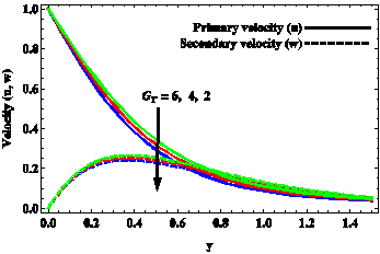
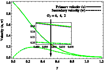
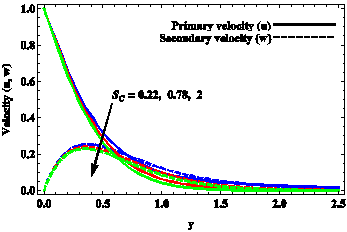
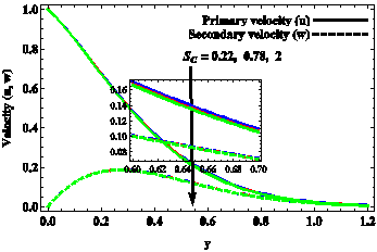
In order to analyze the flow features of the present physical problem, the velocity, temperature and concentration distributions are computed from Eqs (23), (21) and (22) respectively and depicted graphically whereas the skin friction at the plate, Nusselt number and Sherwood number are computed from Eqs (27), (31) and (32) and presented in the tabular form for various values of different pertinent flow parameters taking  $nt=\pi /2\,\,\,\text{and}\,\,\,\varepsilon =1$. In the numerical computations, the boundary condition  $y\to \infty $ is approximated by a maximum value of  $y$ which is sufficiently large for velocity, temperature and concentration to approach their free stream volume. It is observed from Figures (2) to (13) that the fluid velocity in the primary flow direction attains their maximum value at the plate while the fluid velocity in the secondary flow direction attains maximum value in the region near the plate and thereafter these are decreasing on increasing boundary layer parameter  $y$ and approaching to their free stream values.

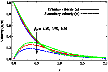
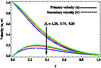
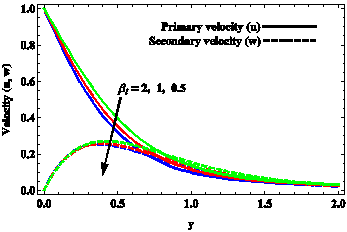
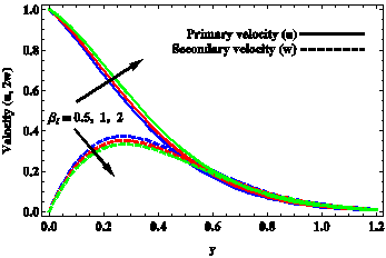
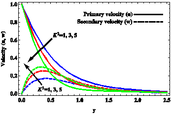
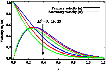
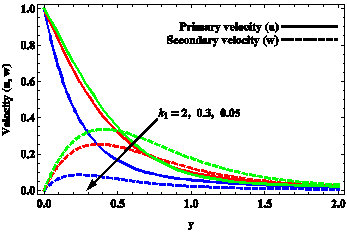
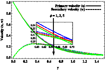
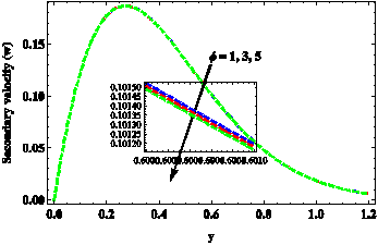
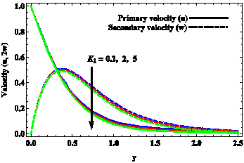
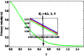
Figures (2) depict variations in velocity distributions versus boundary layer parameter  $y$ for various values of Hall current parameter  ${{\beta }_{e}}$. It is noticed from Figures (2) that the fluid velocity in the primary flow direction increases on increasing  ${{\beta }_{e}}$ near the plate whereas this tendency is reversed in the region away from the plate when  $n<{{X}_{2}}$ while the fluid velocity in the primary flow direction increases on increasing  ${{\beta }_{e}}$ when  $n>{{X}_{2}}$. The fluid velocity in the secondary flow direction increases on increasing ${{\beta }_{e}}$. This shows the fact that the Hall current has tendency to enhance fluid velocity in the primary flow direction in the vicinity of the plate and in the secondary flow direction while it has tendency to reduce the fluid velocity in the primary flow direction in the region away from the plate when natural frequency is greater than the frequency of oscillations. This result agrees with the well established result that Hall current induces fluid flow in the secondary flow direction. Figures (3) represent the velocity distributions for various values of ion-slip parameter  ${{\beta }_{i}}$against boundary layer of parameter  $y$. It is seen from Figures (3) that the fluid velocity in the primary flow direction increases on increasing  ${{\beta }_{i}}$ whereas the fluid velocity in the secondary flow direction increases on increasing  ${{\beta }_{i}}$ when  $n<{{X}_{2}}$ and it decreases on increasing ${{\beta }_{i}}$ when  $n>{{X}_{2}}$. This illustrates the fact the ion-slip has tendency to enhance fluid velocity in the primary flow direction and in the secondary flow direction when the natural frequency is greater than the frequency of oscillations whereas it has tendency to reduce the fluid velocity in the secondary flow direction when the natural frequency is smaller than the frequency of oscillations. Figures (4) show the variations in the velocity distributions verses boundary layer parameter  $y$ for different values of rotation parameter  ${{K}^{2}}$. It is observed from Figures (4) that the fluid velocity in the primary flow direction decreases whereas the fluid velocity in the secondary flow direction increases on increasing  ${{K}^{2}}$. This concludes the fact that the Coriolis force has tendency to reduce fluid velocity in the primary flow direction whereas it has reverse tendency on the fluid velocity in the secondary flow direction. It is well known that Coriolis force induces secondary flow in the flow-field similar to Hall current. Our result is in agreement with it. Figures (5) represent the velocity distributions for various values of magnetic parameter  ${{M}^{2}}$ against boundary layer parameter  $y$. From Figures (5) it is noticed that the fluid velocity in the primary flow direction and the fluid velocity in the secondary flow direction when  $n<{{X}_{2}},$ decrease on increasing  ${{M}^{2}}$ whereas the fluid velocity in the secondary flow direction increases in the vicinity of the plate and it decreases in the region away from the plate on increasing  ${{M}^{2}}$ when  $n>{{X}_{2}}$. This implies that magnetic field (Lorentz force) has tendency to reduce fluid velocity in the primary flow direction and secondary flow direction when the natural frequency is greater than the frequency of oscillations. The magnetic field has tendency to enhance fluid velocity in the secondary flow direction in the vicinity of the plate while this tendency is reversed in the region away from the plate when the natural frequency is smaller than the frequency of oscillations. Similar to the drag force the usual nature of Lorentz force is to suppress the main flow (primary flow), our result agree with it. Figures (6) depict the variations in velocity distributions verses boundary layer parameter $y$ for various values of frequency parameter  $n$. It is evident from Figures (6) that the fluid velocity in the primary flow direction when  $n<{{X}_{2}},$ and the fluid velocity in the secondary flow direction decrease on increasing  $n$ whereas the fluid velocity is the primary flow direction increases in the neighborhood of the plate and it decreases in the region away from the plate on increasing  $n$ when  $n>{{X}_{2}}$. This shows the fact that oscillations has tendency to reduce fluid velocity in the primary flow direction when the natural frequency is greater than the frequency of oscillations and the fluid velocity in the secondary flow direction. Oscillations has tendency to enhance fluid velocity in the primary flow direction in the neighborhood of the plate while this tendency become reverse in the region away from the plate when natural frequency is smaller than the frequency of oscillations. Figures (7) represent the distributions of velocity against boundary layer parameter  $y$ for various values of permeability parameter  ${{k}_{1}}$. Figures (7) demonstrate that the fluid velocity in the primary flow direction when  $n>{{X}_{2}},$ and the fluid velocity in the secondary flow direction increase on increasing  ${{k}_{1}}$ while the fluid velocity in the primary flow direction increases in the vicinity of the plate on increasing  ${{k}_{1}}$ when  $n<{{X}_{2}}$. This illustrates the fact that the Darcian drag force has tendency to reduce fluid velocity in the primary flow direction when natural frequency is smaller than the frequency oscillations and the fluid velocity in the secondary flow direction. Figures (8) and (9) depict variations of velocity distributions versus boundary layer parameter  $y$ for various values of thermal Grashof number  ${{G}_{T}}$ and solutal Grashof number  ${{G}_{C}}$. Figures (8) and (9) exhibit that the fluid velocity in both the primary and secondary flow directions increase on increasing  ${{G}_{T}}\,\,\text{and}\,\,{{G}_{C}}$. This implies that both the thermal and concentration buoyancy forces have tendency to enhance fluid velocity in both the primary and secondary flow directions. In Figures (10) to (13) velocity distributions have been plotted against boundary layer parameter  $y$ for various values of Prandtl number  ${{P}_{r}}$, Schmidt number  ${{S}_{c}}$, heat absorption parameter  $\phi $ and chemical reaction parameter  ${{K}_{1}}$. Figures (10) to (13) display that the fluid velocity in both the primary and secondary flow directions decrease on increasing ${{P}_{r}},\,\,{{S}_{c}},\,\,\phi \,\,\text{and}\,\,{{K}_{1}}$. There is inverse relation of Prandtl number to the thermal diffusion and Schmidt number to the chemical molecular diffusion. This indicates that both the thermal and chemical molecular diffusion have tendency to enhance fluid velocity in the primary and secondary flow directions whereas the heat absorption and chemical reaction have reverse tendency on these.

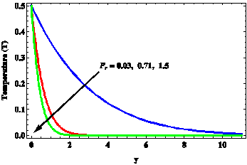
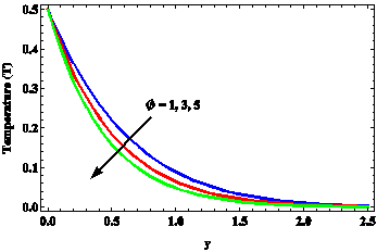
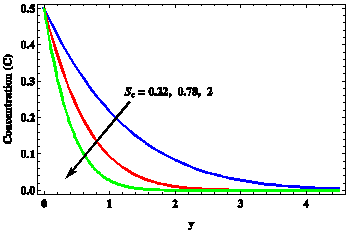
Figures (14) and (15) depict the deviation of temperature distributions versus boundary layer parameter $y$ for various values of  ${{P}_{r}}$ and  $\phi $ while Figures (16) and (17) represent the variation of concentration distributions versus boundary layer parameter  $y$ for various values of  ${{S}_{c}}$ and  ${{K}_{1}}$. It is noticed from Figures (14) and (15) that fluid temperature decreases with increase in  ${{P}_{r}}$ and  $\phi $ while Figures (16) and (17) display that concentration decreases with increase in  ${{S}_{c}}$ and  ${{K}_{1}}$. This shows that thermal diffusion enhances fluid temperature while heat absorption shows the reverse influence on it. Chemical molecular diffusion give rise in species concentration while chemical reaction shows reverse tendency on it.

It is also noted from Figures (10) and (14) that the thicknesses of momentum and thermal boundary layers decrease with increase in  ${{P}_{r}}$. Figures (11) and (16) demonstrate that the thicknesses of momentum and concentration boundary layers decrease with increase in  ${{S}_{c}}$. It means that thermal diffusion give rise in momentum and thermal boundary layer thicknesses while chemical molecular diffusion shows the similar influence on momentum and concentration boundary layer thicknesses.

Tables (2) represents the variation of skin friction in the primary and secondary flow directions for varies values of ${{\beta }_{e}}$ and ${{\beta }_{i}}$. It is revealed from Tables (2) that the skin friction in the primary flow direction decreases on increasing both ${{\beta }_{e}}$ and ${{\beta }_{i}}$ whereas the skin friction in secondary flow direction increases on increasing ${{\beta }_{e}}$ and it decreases on increasing ${{\beta }_{i}}$ when ${{\beta }_{e}}=0.75\,\,\text{and}\,\,1.25$. This shows that both the Hall current and ion-slip have tendency to reduce skin friction in the primary flow direction whereas Hall current has tendency to enhance skin friction in the secondary flow direction while ion-slip has reverse tendency on it when ${{\beta }_{e}}=0.75\,\,\text{and}\,\,1.25$. Tables (3) describe the variation of skin friction in the primary and secondary flow directions for varies values of ${{K}^{2}}$ and ${{M}^{2}}$. It is illustrated from Tables (3) that the skin friction in both the primary and secondary flow directions increase on increasing both ${{K}^{2}}$ and ${{M}^{2}}$. This implies the fact that both the Coriolis force and Lorentz force have tendency to enhance skin friction in both the primary and secondary flow directions. Tables (4) depict the distributions of skin friction in the primary and secondary flow directions for varies values of $n\,\,\text{and}\,\,{{k}_{1}}$. It is noticed from Tables (4) that the skin friction in the primary flow direction decreases whereas the skin friction in the secondary flow direction increases on increasing ${{k}_{1}}$. The skin friction in the primary flow direction decreases on increasing $n$ when $n>{{X}_{2}}$. The skin friction in the primary flow direction increases, attains a maximum value and again decreases on increasing $n$ when $n<{{X}_{2}}$ while this tendency become reverse on the skin friction in the secondary flow direction when $n<{{X}_{2}}$. This shows the fact that the Darcian drag force has tendency to enhance skin friction in the primary flow direction whereas it has reverse tendency on the skin friction in the secondary flow direction. Oscillations has tendency to reduce skin friction in the primary flow direction when natural frequency is smaller than frequency of oscillations. Tables (5) represents the distributions of skin friction in the primary and secondary flow directions for various values of  ${{G}_{T}}$ and ${{G}_{C}}$. It is observed from Tables (5) that the skin friction in the primary flow direction decreases whereas the skin friction in the secondary flow direction increases on increasing both ${{G}_{T}}$ and  ${{G}_{C}}$. This indicates the fact that both the thermal and concentration buoyancy forces have tendency to reduce skin friction in the primary flow direction where as these have reverse tendency on skin friction in the secondary flow direction. Tables (6) represent the variations of skin friction in the primary and secondary flow directions for varies values of ${{P}_{r}}$ and  ${{S}_{c}}$. It is revealed from Tables (6) that the skin friction in the primary flow direction increases whereas skin friction in the secondary flow direction decreases on increasing both ${{P}_{r}}$ and ${{S}_{c}}$. This shows that both the thermal and chemical molecular diffusions have tendency to reduce skin friction in the primary flow direction whereas these have reverse tendency on the skin friction in the secondary flow direction. Tables (7) display the distributions of skin friction in primary and secondary flow directions for various values of $\phi $ and ${{K}_{1}}$. It is illustrated from Tables (7) that the skin friction in the primary flow direction increases on increasing both $\phi $ and ${{K}_{1}}$ whereas the skin friction in the secondary flow direction decreases on increasing ${{K}_{1}}$ while it increases on increasing $\phi $ when $n>{{X}_{2}}$ and it decreases on increasing $\phi $ when $n<{{X}_{2}}$. This reveals that both the heat absorption and chemical reaction have tendency to enhance skin friction in the primary flow direction. The chemical reaction has tendency to reduce skin friction in the secondary flow direction whereas the heat absorption has tendency to enhance the skin friction in the secondary flow direction when natural frequency is smaller than frequency of oscillations while this tendency is reversed when natural frequency is greater than the frequency of oscillations.

Tables (8) and (9) show the variations of heat and mass transfer at the plate in terms of Nusselt and Sherwood numbers respectively. It is clear from Tables (8) and (9) that Nusselt number  $Nu$ increases with increase in both  ${{P}_{r}}$ and  $\phi $ while Sherwood number  $Sh$ increases with increase in both  ${{S}_{c}}$ and  ${{K}_{1}}$. This reflects that thermal diffusion reduces rate of heat transfer of the plate while heat absorption shows the reverse influence on it. Chemical molecular diffusion reduces rate of mass transfer at the plate while chemical reaction shows the reverse trend on it.

2a.png

(a) $n=3$

2b.png

(b) $n=15$

Figure 2. Velocity distributions for (a) $n<{{X}_{2}}$ and (b) $n>{{X}_{2}}$, when  ${{\beta }_{i}}=0.5,\,\,{{K}^{2}}=3,\,\,{{M}^{2}}=9,\,\,{{k}_{1}}=0.3,\,\,{{G}_{T}}=4,$  ${{G}_{C}}=5,\,\,{{P}_{r}}=0.71,\,\,{{S}_{c}}=0.22,\,\,\,\phi =1\,\,\text{and}\,{{K}_{1}}=0.2.$

3a.png

(a) $n=3$

3b.png

(b) $n=15$

Figure 3. Velocity distributions for (a) $n<{{X}_{2}}$ and (b) $n>{{X}_{2}}$ when  ${{\beta }_{e}}=0.75,\,\,{{K}^{2}}=3,\,\,{{M}^{2}}=9,\,\,{{k}_{1}}=0.3,\,\,{{G}_{T}}=4,$ ${{G}_{C}}=5,\,\,{{P}_{r}}=0.71,\,\,{{S}_{c}}=0.22,\,\,\,\phi =1\,\,\text{and}\,{{K}_{1}}=0.2.$

4a.png

(a) $n=3$

4b.png

(b) $n=15$

Figure 4. Velocity distributions for (a) $n<{{X}_{2}}$ and (b) $n>{{X}_{2}}$ when  ${{\beta }_{e}}=0.75,\,\,{{\beta }_{i}}=0.5,\,\,{{M}^{2}}=9,\,\,{{k}_{1}}=0.3,\,\,{{G}_{T}}=4,$ ${{G}_{C}}=5,\,\,{{P}_{r}}=0.71,\,\,{{S}_{c}}=0.22,\,\,\,\phi =1\,\,\text{and}\,{{K}_{1}}=0.2.$

5a.png

(a) $n=3$

5b.png

(b) $n=15$

Figure 5. Velocity distributions for (a) $n<{{X}_{2}}$ and (b) $n>{{X}_{2}}$ when  ${{\beta }_{e}}=0.75,\,\,{{\beta }_{i}}=0.5,\,\,{{K}^{2}}=3,\,\,{{k}_{1}}=0.3,\,\,{{G}_{T}}=4,$ ${{G}_{C}}=5,\,\,{{P}_{r}}=0.71,\,\,{{S}_{c}}=0.22,\,\,\,\phi =1\,\,\text{and}\,{{K}_{1}}=0.2.$

6a.png

(a) $n=3$

6b.png

(b) $n=15$

Figure 6. Velocity distributions for (a) $n<{{X}_{2}}$ and (b) $n>{{X}_{2}}$ when  ${{\beta }_{e}}=0.75,\,\,{{\beta }_{i}}=0.5,\,\,\,{{K}^{2}}=3,\,\,\,{{M}^{2}}=9,\,\,{{G}_{T}}=4,$ ${{G}_{C}}=5,\,\,{{P}_{r}}=0.71,\,\,{{S}_{c}}=0.22,\,\,\,\phi =1\,\,\text{and}\,{{K}_{1}}=0.2.$

7a.png

(a) $n=3$

7b.png

(b) $n=15$

Figure 7. Velocity distributions for (a) $n<{{X}_{2}}$ and (b) $n>{{X}_{2}}$ when  ${{\beta }_{e}}=0.75,\,\,{{\beta }_{i}}=0.5,\,\,\,{{K}^{2}}=3,\,\,\,{{M}^{2}}=9,\,\,{{G}_{T}}=4,$ ${{G}_{C}}=5,\,\,{{P}_{r}}=0.71,\,\,{{S}_{c}}=0.22,\,\,\,\phi =1\,\,\text{and}\,{{K}_{1}}=0.2.$

8a.png

(a) $n=3$

8b.png

(b) $n=15$

Figure 8. Velocity distributions for (a) $n<{{X}_{2}}$ and (b) $n>{{X}_{2}}$ when  ${{\beta }_{e}}=0.75,\,\,{{\beta }_{i}}=0.5,\,\,\,{{K}^{2}}=3,\,\,\,{{M}^{2}}=9,\,{{k}_{1}}=0.3,$ ${{G}_{C}}=5,\,\,{{P}_{r}}=0.71,\,\,{{S}_{c}}=0.22,\,\,\,\phi =1\,\,\text{and}\,\,{{K}_{1}}=0.2.$

9a.png

(a) $n=3$

9b.png

(b) $n=15$

Figure 9. Velocity distributions for (a) $n<{{X}_{2}}$ and (b) $n>{{X}_{2}}$ when  ${{\beta }_{e}}=0.75,\,\,{{\beta }_{i}}=0.5,\,\,\,{{K}^{2}}=3,\,\,\,{{M}^{2}}=9,\,\,{{k}_{1}}=0.3,$ ${{G}_{T}}=4,\,\,{{P}_{r}}=0.71,\,\,{{S}_{c}}=0.22,\,\,\phi =1\,\,\text{and}\,\,{{K}_{1}}=0.2.$

10a.png

(a) $n=3$

10b.png

(b) $n=15$

Figure 10. Velocity distributions for (a) $n<{{X}_{2}}$ and (b) $n>{{X}_{2}}$ when  ${{\beta }_{e}}=0.75,\,\,{{\beta }_{i}}=0.5,\,\,\,{{K}^{2}}=3,\,\,\,{{M}^{2}}=9,\,\,{{k}_{1}}=0.3,$ ${{G}_{T}}=4,\,\,{{G}_{C}}=5,\,\,\,{{S}_{c}}=0.22,\,\,\,\phi =1\,\,\text{and}\,\,{{K}_{1}}=0.2.$

11a.png

(a) $n=3$

11b.png

(b) $n=15$

Figure 11. Velocity distributions for (a) $n<{{X}_{2}}$ and (b) $n>{{X}_{2}}$ when  ${{\beta }_{e}}=0.75,\,\,{{\beta }_{i}}=0.5,\,\,\,{{K}^{2}}=3,\,\,\,{{M}^{2}}=9,\,\,{{k}_{1}}=0.3,$ ${{G}_{T}}=4,\,\,{{G}_{C}}=5,\,\,\,{{P}_{r}}=0.71\,,\,\,\,\phi =1\,\,\,\text{and}\,\,{{K}_{1}}=0.2.$

12a.png

(a) $n=3$

12ba.png

12bb.png

(b) $n=15$

Figure 12. Velocity distributions for (a) $n<{{X}_{2}}$ and (b) $n>{{X}_{2}}$ when  ${{\beta }_{e}}=0.75,\,\,{{\beta }_{i}}=0.5,\,\,\,{{K}^{2}}=3,\,\,\,{{M}^{2}}=9,\,\,{{k}_{1}}=0.3,$ ${{G}_{T}}=4,\,\,{{G}_{C}}=5,\,\,{{P}_{r}}=0.71,\,\,{{S}_{c}}=0.22\,\,\text{and}\,\,{{K}_{1}}=0.2.$

13a.png

(a) $n=3$

13ba.png

13bb.png

(b) $n=15$

Figure 13. Velocity distributions for (a) $n<{{X}_{2}}$ and (b) $n>{{X}_{2}}$ when  ${{\beta }_{e}}=0.75,\,\,{{\beta }_{i}}=0.5,\,\,\,{{K}^{2}}=3,\,\,\,{{M}^{2}}=9,\,\,{{k}_{1}}=0.3,$ ${{G}_{T}}=4,\,\,{{G}_{C}}=5,\,\,{{P}_{r}}=0.71\,,\,\,\,{{S}_{c}}=0.22\,\,\,\,\text{and}\,\,\phi =1\,.$

14.png

Figure 14. Temperature distributions when $\phi =1$.

15.png

Figure 15. Temperature distributions when ${{P}_{r}}=0.71$.

16.png

Figure 16. Concentration distributions when ${{K}_{1}}=0.2$.

17.png

Figure 17. Concentration distributions when ${{S}_{c}}=0.22$.

Table 2. Skin friction distributions for (a) $n<{{X}_{2}}$ and (b) $n>{{X}_{2}}$ when  ${{K}^{2}}=3,\,\,{{M}^{2}}=9,\,\,{{k}_{1}}=0.3,\,\,{{G}_{T}}=4,\,\,{{G}_{C}}=5,$ ${{P}_{r}}=0.71,\,\,{{S}_{c}}=0.22,\,\,\,\phi =1\,\,\text{and}\,\,{{K}_{1}}=0.2.$

(a) $n=3$

(b) $n=15$

Table 3. Skin friction distributions for (a) $n<{{X}_{2}}$and (b)  $n>{{X}_{2}}$when ${{\beta }_{e}}=0.75,\,\,\,{{\beta }_{i}}=0.5,\,{{k}_{1}}=0.3,\,\,{{G}_{T}}=4,\,\,{{G}_{C}}=5,$ ${{P}_{r}}=0.71,\,\,\,{{S}_{c}}=0.22,\,\,\,\phi =1\,\,\text{and}\,\,{{K}_{1}}=0.2.$

(a) $n=3$

(b) $n=15$

Table 4. Skin friction distributions for (a) $n<{{X}_{2}}$ and (b) $n>{{X}_{2}}$ when $\,{{\beta }_{e}}=0.75,\,\,{{\beta }_{i}}=0.5,\,\,{{K}^{2}}=3,\,\,{{M}^{2}}=9,\,\,{{G}_{T}}=4,$ ${{G}_{C}}=5,\,\,{{P}_{r}}=0.71,\,\,{{S}_{c}}=0.22,\,\,\phi =1\,\,\text{and}\,\,{{K}_{1}}=0.2.$

(a) $n=3$

(b) $n=15$

Table 5. Skin friction distributions for (a) $n<{{X}_{2}}$ and (b) $n>{{X}_{2}}$ when $\,{{\beta }_{e}}=0.75,\,\,{{\beta }_{i}}=0.5,\,\,{{K}^{2}}=3,\,\,{{M}^{2}}=9,\,\,{{k}_{1}}=0.3,$ ${{P}_{r}}=0.71,\,\,{{S}_{c}}=0.22,\,\,\phi =1\,\,\text{and}\,\,{{K}_{1}}=0.2.$

(a) $n=3$

(b) $n=15$

Table 6. Skin friction distributions for (a) $n<{{X}_{2}}$ and (b) $n>{{X}_{2}}$ when ${{\beta }_{e}}=0.75,\,\,{{\beta }_{i}}=0.5,\,\,{{K}^{2}}=3,\,\,{{M}^{2}}=9,\,\,{{k}_{1}}=0.3,$ ${{G}_{T}}=4,\,\,{{G}_{C}}=5,\,\,\phi =1\,\,\text{and}\,\,{{K}_{1}}=0.2.$

(a) $n=3$

(b) $n=15$

Table 7. Skin friction distributions for (a) $n<{{X}_{2}}$ and (b) $n>{{X}_{2}}$ when ${{\beta }_{e}}=0.75,\,\,\,{{\beta }_{i}}=0.5,\,\,{{K}^{2}}=3,\,\,{{M}^{2}}=9,\,\,{{k}_{1}}=0.3,$ ${{G}_{T}}=4,\,\,{{G}_{C}}=5,\,\,{{P}_{r}}=0.71\,\,\text{and}\,\,{{S}_{c}}=0.22.$

(a) $n=3$

(b) $n=15$

Table 8. Nusselt number

Table 9. Sherwood number

Authors P. Rohidas [File No: F1-17.1/2016-17/RGNF-2015-17-SC-KAR-10391/(SA-III/Website)] and S. G. Begum [File No: F1-17.1/2014-15/MANF-2014-15-MUS-KAR35378/(SA-III/Website)] are thankful to University Grant Commission (UGC), New Delhi (India) for providing Junior Research Fellowship to carry out this research work.