OPEN ACCESS
The exergetic analysis, a thermodynamics methodology that quantifies Exergy losses associated with irreversibility, allows to optimize each stage of a transformation process and thus its overall efficiency.
In this contribution, a novel approach to exergetic analysis is applied to energy transformations taking place within the core of a nuclear reactor. To perform such analysis, reference was made to a pressurized light-water reactor (PWR), modeling heat exchanges between fuel assemblies and coolant fluid in the core by balancing incoming and outgoing mass and energy flows, incoming and outgoing in the reactor. Analysis results are validated through a comparison with actual reactor operating parameters.
Main goals of the work –part of a wider ongoing research effort- are to develop the thermo-economic analysis of a PWR nuclear power plant (NPP) to assess the actual cost of the products obtainable downstream of the NPP (electric energy and thermal energy for industrial and civil users, very different products in terms of exergy contents), and to compare such costs those of similar products obtained from conventional thermal power plants.
Exergy analysis, Energy conversion, Thermodynamic simulation, PWR reactor, Fission energy.
For many decades processes taking place in complex systems such as thermal power plants have been based on a traditional thermodynamic analysis considering energy and mass conservation. The First Law, however, is not sufficient to accurately evaluate the performance of such systems: in fact, during all real processes entropy is produced due to irreversibility of energy transformations. As regards efficiency evaluation of a thermal system doing work it is necessary to deal with all sources of thermodynamic ineffectiveness: to this end, exergy turns out to be the optimal measure system [1].
In thermodynamics, given a certain amount of total energy, exergy is defined as the maximum useful work at the end of the transformation process; as a consequence, exergy allows to evaluate energy degradation associated with the process due to irreversibilities (exergy is conserved only in the case of reversible, ideal process) [21].
One of the most relevant characteristic of the exergy concept is its huge versatility, because it is possible to estimate fluxes and balances of any kind of energy for each element of a complex system, using a simple efficiency criterion [15, 25]. Moreover, the exergy concept can be usefully utilized for technical and economic analyses aimed at optimization of a process (thermo-economic analysis) and/or for a more efficient energy use (exergo-environmental analysis) [17,18, 26].
To date, despite the undisputed usefulness of the concept of exergy in the context of process optimization, energy analyses performed in the design of industrial installations never include evaluation of the exergetic efficiency. It is true that, since the 50s, a significant research activity has been carried out and that, in some applications, also exergy efficiency of a nuclear power plant was analyzed. In such works, however, the nuclear reactor was always modelled as a simple black box, taking into account only coolant inlet and outlet temperatures and reactor core thermal power [9,16].
In this paper, a detailed exergetic analysis of a pressurized water reactor (PWR) is carried out in order to define more accurately its exergetic efficiency. The results are compared with the average data obtained in literature, and used to create an exergetic core model that can support other design tools (thermal design, hydraulic design, mechanical design, neutronic design) in order to optimize the nuclear reactor also in terms of exergy efficiency [8,12,13].
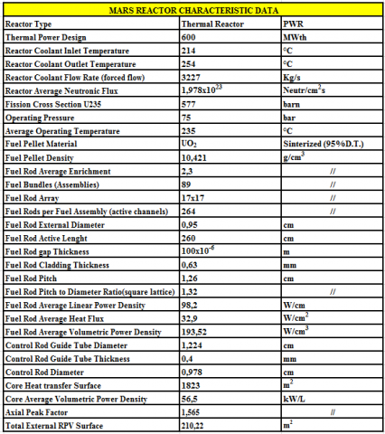
In order to quantify the results of the modeling, the design characteristics of MARS Reactor (Multipurpose Advanced Reactor inherently Safe) has been assumed as reference.
The MARS Reactor, a Pressurized Water Reactor designed in the 80s at the Department of Nuclear Engineering and Energy Conversion of Sapienza University of Rome, represents a new concept of inherently safe reactor, which can be used for a wide range of applications, from electricity production to district heating and desalination, as well as other products [4]. Designed for a nuclear power generation capacity of about 600MWth, corresponding to about 170 MWe in the case of only electrical production, the MARS Reactor is classified among the Small Modular Reactors (SMRs), a new generation of modular nuclear power plants developed to provide flexible, cost-effective energy for various applications, with specific safety features that allow it to be positioned near towns or industrial areas.
Table 1 presents the most important MARS characteristic data, utilized for the numerical application of the modeling. The section of the reactor pressure vessel (RPV) is shown in Figure 1 [4, 5, 6].
Table 1. MARS characteristic data [4, 5]
Figure 1. MARS reactor schemes
3.1 Thermodynamic theoretical equations
Considering a reactor operating in steady-state as an open system, the exergetic analysis is based on the four balances outlined in Fig. 2, and in the following corresponding equations [2, 7].
Figure 2. Thermodynamic balances [2, 7 ]
Σin ṁ = Σout ṁ (Mass balance)(i)
Σin ṁ (h+ gz + w2/2) +$\dot{Q}$= Ĺ+ Σout ṁ (h+ gz + w2/2) (Energy balance)(ii)
Σin | $\dot{Q}$ /T|+ Σin ṁ s + Śgen = Σout | $\dot{Q}$ /T| + Σout ṁ s (Entropy balance)(iii)
Σin ṁ ex + Σ Ėxq - Ėxδ = Ĺ + Σout ṁ ex (Exergy balance)(iiii)
To obtain at a glance the definition of exergetic efficiency, it is useful to resort to the Grassmann diagram shown in Fig.3, together with the exergetic efficiency formula [10, 11, 14, 22].
Figure 3. Exergetic efficiency formula [11]
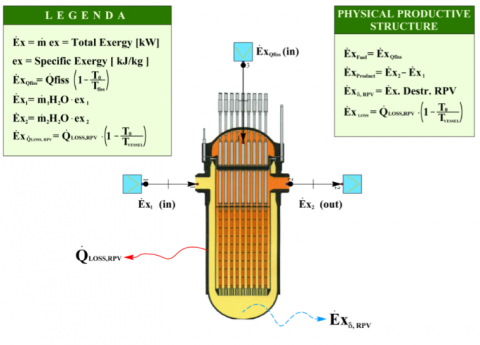
3.2 Mathematical modeling of the reactor
Fig. 4 illustrates the exergetic modeling of a pressurized water reactor, in perfect analogy to Fig. 3.
Figure 4. MARS reactor exergy balances
Referring to this figure, the theoretical equations of the thermodynamics are applied as follows:
$\dot{m}_{1}=\dot{m}_{2}$(1)
$\dot{m}_{1} h_{1}+\dot{Q}_{f i s s}-\dot{Q}_{l o s s}=\dot{m}_{1} h_{2}$(2)
$\dot{m}_{1} s_{1}+\frac{\dot{Q}_{f i s s}}{T_{f i s s}}+\frac{\dot{Q}_{l o s s}}{T_{V e s s}}+\dot{S}_{g e n}=\dot{m}_{1} s_{2}$(3)
$\dot{m}_{1} e x_{1}+\dot{E} x_{f i s s}-\dot{E} x_{l o s s}-\dot{E} x_{\delta R P V}=\dot{m}_{1} e x_{2}$(4)
for the Exergy Efficiency [10,14]:
$\varepsilon_{R P V}=1-\frac{\dot{E} x_{l o s s}+\dot{E} x_{\delta R R V}}{\dot{E} x_{\varrho f s s}}$(5)
in which:
$\dot{E} x_{Q f s s}=\dot{Q}_{f i s s}\left(1-\frac{T_{0}}{T_{f i s s}}\right)$(6)
$\dot{E} x_{l o s s}=\dot{Q}_{l o s s}\left(1-\frac{T_{0}}{T_{V e s s}}\right)$(7)
$\dot{E} x_{\delta R P V}=\dot{E} x_{\varrho f s s}-\dot{E} x_{P}-\dot{E} x_{l o s s}$(8)
To carry out the exergetic analysis of the reactor, the following simplifying hypotheses are assumed:
1) steady-state operation mode;
2) average constant enrichment of all fuel rods in the core, equal to 2.3%;
3) net energy for each fission equal to 200 MeV;
4) coolant mass flow homogeneously divided in each fuel rod;
5) constant cp value of the coolant water around each fuel rod (it increases by about 7% between the top and the bottom of the core) and equal to 4.74kJ/kg K;
6) reference condition for each exergy assessment: P0=101.3 [kPa]; T0=298.15 [K]; s0=0.367 [kJ / kg K]; h0=104.93 [kJ / kg].
With reference to the fuel exergy as estimated in equation (6), the following steps are performed :
${{q}^{'''}}\,={{E}_{fiss}}\,{{\sigma }_{fiss}}\,{{\Phi }_{n}}\,{{\rho }_{UO2}}\,\,\,\frac{{{N}_{A}}}{{{M}_{UO2}}(\bar{X})}\,\bar{X}$ (9)
${{\dot{Q}}_{fiss}}$=${{q}^{'''}}$Vf (10)
To simulate the axial temperature shape of the cooling water, the following expression is used:
$T_{H 2 O}(z)=T_{H 2 o i n}+\frac{q_{\max }^{\prime} H_{e}}{\pi \overline{c}_{p H 2 O} \dot{m}_{H 2 O}} \times\left[\operatorname{sen}\left(\frac{\pi z}{H_{e}}\right)+\operatorname{sen}\left(\frac{\pi H a}{2 H_{e}}\right)\right]$(11)
To solve such an expression the linear power density q'max and the extrapolated fuel rod height, He, (at which neutron flux is equal to zero) are required.
To obtain q’max, the linear heat flux at the center of the rod height, as illustrated in Fig 5, the following expression is used [6]:
${{T}_{H2O}}(z)\,=\,{{T}_{H2O}}_{in\,}+\,\frac{q{{'}_{\max }}\,{{H}_{e}}_{\,}}{\pi \,{{{\bar{c}}}_{pH2O}}\,{{{\dot{m}}}_{H2O}}}\,\times \,\left[ sen\,\ \left( \frac{\pi \,z}{{{H}_{e}}}\, \right)+sen\ \,\left( \frac{\pi \,Ha}{2{{H}_{e}}} \right) \right]\,\,$ (12)
Figure 5. Linear heat flux for a PWR reactor
Since all the parameters of interest are axially symmetric, as evident from Fig. 5, in all the simulations the origin of the reference axes has always been positioned at the center of the rod at its half height.
To obtain the extrapolated fuel rod height, He, the following expression can be used [6]:
$H_{e}=H_{a}+2 \delta=H_{a}+2 \frac{0.71}{\Sigma_{n}}$(13)
in which δ is the adjunctive length necessary to obtain the correct position of the zero neutronic flux boundary condition, and Str is the macroscopic transport cross section.
This quantity is equal to the macroscopic total cross section multiplied by the transport factor ($1-\overline{\mu}_{0}$) [3]:
$\Sigma_{\mathrm{tr}}=\Sigma_{\mathrm{tot}}\left(1-\overline{\mu}_{0}\right)$(14)
Stot can be calculated in terms of the middle temperature of the coolant water, $\overline{T}_{H 2 O}$ , as it follows:
$\Sigma_{t o t}=N_{H 2 O}\left(\overline{T}_{H 2 O}\right)\left[\sigma_{d b s}\left(\overline{T}_{H 2 O}\right)+\sigma_{s c}\left(\overline{T}_{H 2 O}\right)\right]$(15)
in which (T0 = 293.15 K and TH2O = 235°C):
$\sigma(\overline{T})=\sigma_{0} \sqrt{\frac{T_{0}}{\overline{T}}}$(16)
Figure 6. Sub-channel temperature profile for a PWR reactor
With the above relationships it is possible to estimate the cooling water temperature profile along the sub channel around a fuel rod and, referring to a general shape as showed in Fig. 6, it is possible to go back to the central temperature of a fuel rod.
Knowing the temperature of the coolant water, TH20(z), the convective heat transfer coefficient for water flowing parallel to the clad can be calculated by means of the Weisman correlation (describing a single-phase forced convection in turbulent regime):
$N u=C R_{e}^{0.8} P_{r}^{1 / 3}$(17)
in which C is a function of the pitch-to-diameter ratio of a single subchannel [27].
With this correlation the convective heat transfer coefficient for turbulent water can be obtained as follows:
$h_{\text {wall}}=\frac{N u K_{H 2 O}}{D_{e}}$(18)
and the wall temperature, which is the external temperature of the clad, can be obtained from the following equation:
$q^{\prime \prime}=h_{w a l l}\left(T_{w a l l}-T_{H 2 O}\right)$(19)
The internal temperature of the clad, $T_{g i}$ , assuming the Zircaloy conductivity as a constant along the axis, can be assessed using the Fourier equation:
$q^{\prime}=\frac{2 \pi K_{z i r c}}{\ln \left(R_{e s t} / R_{g}\right)}\left(T_{g i}-T_{w a l l}\right)$(20)
The external temperature of the fuel pellet, $T_{S}$ , depends upon the thermal conductivity of the Helium in the gap. Helium is supposed to be stagnant, at an intermediary temperature among TS and Tgi. The Zircaloy conductivity correlation used in the work (heat transfer for radiation is neglected) is the following [20]:
$K_{H e}=0.144\left[1+2.7 \times 10^{-4} p_{H e}\left(T_{H e} / T_{o}\right)\right]^{0.71\left(1-2 \times 10^{-4} p_{B e}\right)}$(21)
in which: T0 = 273.15 K and pHe = 11,25 bar;
TS is calculated by means of an iterative application of the Fourier equation in the following terms [6,27]:
$q^{\prime}(z)=\frac{2 \pi K_{H e}}{\ln \left(R_{p} / R_{g}\right)}\left(T_{S}-T_{g i}\right)$(22)
Knowing TS, the central temperature of the fuel rod, can be calculated by means of the Integral Conductivity correlation which only depends on the characteristic of the fuel and on the temperature Tc at the center of the rod:
$q^{\prime}(z)=4 \pi I . C .=4 \pi \int_{T_{s}}^{T_{c}} K_{U O 2}(T) d T$(23)
in which [23]:
$K_{U O 2}(T)=\frac{100}{6.548+23.533\left(\frac{T}{10^{3}}\right)}+\frac{6400}{\left(\frac{T}{10^{3}}\right)^{5 / 2}} \exp ^{\left(\frac{-16.35}{T / 0^{3}}\right)}$(24)
Tc is calculated along the fuel rod axis by means of an iterative application of the above mentioned equations along the active rod height thus obtaining the Tc(z) profile.
Finally Tfiss is evaluated as the average value of the Tc(z) curve among the top and the bottom of the fuel rod.
With reference to Exergy losses as estimated in equation (7), $\dot{Q}_{\text {loss}}$ , and therefore $\dot{E} x_{l o s s}$ , are easily found, knowing PRV geometrical dimensions, steal heat thickness and conductivity and reference containment temperature.
At this point of the modeling all data are available to calculate $\dot{E} x_{\delta}$ using equation (8) and, therefore, the reactor Exergy Efficiency using equation (5).
The mathematical model described so far is now applied to verify the MARS exergetic efficiency, with reference to data in Tab. 1.
First, in Tab 2 and Fig. 7 fuel rod central temperature, Tc, evaluated at 10 cm- step up and down the central quote, is presented.
Table 2. MARS fuel rod central temperature profile (data plotted in Figure 7)
Figure 7. MARS fuel rod central temperature profile (data listed in Table 2)
From the above simulation Tfiss can be obtained as the average arithmetic value obtaining 1028.2 K.
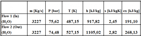
Table 3. MARS coolant main thermodynamic data [24]
Using the values of the parameters reported in Table 1 and in Table 3, and the above mentioned equations, all the main results are found as follows:
$\dot{Q}_{\text {fiss}}$ = 606.2 MWth and $\dot{E} x_{Q f s s}=\dot{E} x_{F}=$ 430.42 MWth
$\dot{Q}_{\text {lossRPV}}$= 2.1 MWth (mainly bare vessel thermal dispersion)
and $\dot{E} x_{l o s s}$ = 0.87 MWth
Referring to $\dot{E} x_{P}$ , it is possible to write:
$\dot{E} x_{P}=\dot{m}\left(e x_{2}-e x_{1}\right)=248.8$ MWth
in which, referring to data in table 2:
$e x_{i}=\left(h_{i}-h_{0}\right)-T_{0}\left(s_{i}-s_{0}\right)$(25)
Therefore,
$\dot{E} x_{\delta R P V}=\dot{E} x_{Q f i s s}-\dot{E} x_{P}-\dot{E} x_{l o s s}$= 430.42 – 248.8 – 0.87= 181 MWth
and finally:
$\varepsilon=\frac{\dot{E} x_{P}}{\dot{E} x_{F}}=57.8$ %
Modeling results confirm the order of magnitude obtained by other researches in which the reactor, analyzed as a black box inside the equipment of a nuclear power plant, is proved to have exergetic efficiencies always between 50 and 60 %. This efficiency range once again shows that the nuclear reactor presents a second law efficiency approximately equal to that of a traditional combustion chamber.
Next step of the present work – in the frame of a wider ongoing research - is to develop the thermo-economic analysis of a PWR nuclear power plant in order to assess the actual cost of products obtainable downstream of the plant (electric energy and thermal energy useful for industrial and civil users, very different products in terms of exergy contents), and compare them with the costs of similar products obtained from conventional thermal power plants.
The final goal of the research is to create a whole exergetic model of the entire primary PWR loop that can support other design tools (thermal, hydraulic, mechanical and neutronic design) in order to optimize the nuclear reactor loop also in terms of exergy efficiency.
|
$\dot{E} x$ |
total Exergy, kW |
|||
|
$\dot{E} x_{\delta}$ |
total Exergy destruction, kW |
|||
|
$\dot{Q}$ |
heat transfer rate, kW |
|||
|
$\dot{S}$ |
total Entropy, kW.K-1 |
|||
|
$\dot{S}_{\text { gen }}$ |
total Entropy generation, kW |
|||
|
ex |
specific Exergy, kJ.kg-1 |
|||
|
s |
specific Entropy, kJ. specific Entropy, kJ.kg-1.K-1 |
|||
|
h |
specific Entalpy, kJ.kg-1. |
|||
|
$\dot{m}$ |
mass flow rate, kg.s-1 |
|||
|
p |
pressure, Pa |
|||
|
T |
temperature, K |
|||
|
V |
volume, m3 |
|||
|
v |
specific volume, m3.kg-1 |
|||
|
w |
velocity, m.s-1 |
|||
|
NA |
Avogadro’s number |
|||
|
M |
molecular weight, g.mole-1 |
|||
|
Subscripts |
|
|||
|
f |
fuel |
|||
|
fiss |
fission |
|||
|
RPV |
Reactor pressure vessel |
|||
|
gen |
generated |
|||
|
tr |
transport |
|||
|
δ |
destruction |
|||
|
loss Vess |
loss, released to the environment RPV external surface |
|||
|
$\overline{X}$ N |
average fuel enrichement atomic density, cm-3 |
|||
|
FPA L Efiss |
axial peak factor work, kW fission energy, J |
|||
|
K |
thermal conductivity, W.cm-1.K-1 |
|||
|
De |
subchannel equivalent diameter, cm |
|||
|
G |
specific mass flow rate, kg.cm-2.s-1 |
|||
|
$\overline{C}_{p}$ |
average isobaric specific heat, J.kg-1.k-1 |
|||
|
$q^{\prime}$ |
linear power density, W.cm-1 |
|||
|
$q^{\prime \prime}$ |
heat flux, W.cm-2 |
|||
|
$q^{\prime \prime \prime}$ |
volumetric power density, W.cm-3 |
|||
|
$H_{a}$ |
active rod length, cm |
|||
|
$H_{e}$ |
extrapolated rod length, cm |
|||
|
He |
Helium Gas |
|||
Greek symbols
|
δ |
adjunctive lenght [used in eq. (13)], cm |
|
ρ |
density, kg.m-3 |
|
ε |
Exergetic efficiency Exergetic efficiency |
|
σ |
microscopic cross section, cm2 |
|
Φn |
neutronic flux, cm-2.s-1 |
|
$\sum$ |
macroscopic cross section, cm-1 |
|
$\overline{\mu}_{0}$ |
average cosin of the scattering angle |
|
$\mu$ |
dynamic viscosity, P dynamic viscosity, Pa.s |
[1] Sciubba E., Wall G.,”A brief commented History of Exergy from Beginnings to 2004” International Journal of Thermodynamics, vol. 10, no. 1, pp. 1-26, March 2007.
[2] R. Mastrullo, P. Mazzei and R. Vanoli, Fondamenti di Energetica, Napoli, Italy: Liguori, Ed.1992 , pp. 9-95.
[3] S. Sciuti and D. Borsani, Tabelle e grafici per calcoli di fisica nucleare applicata all'ingegneria, alla chimica ed alla medicina, Roma, Italy: Libreria Eredi V.Veschi, Ed.1984, pp. 18-19.
[4] DINCE, University of Rome, 600 MWth MARS NPP Design Progress Report 2003, Roma, Italy, 2003.
[5] M.Cumo, Impianti Nucleari, Roma, Italy: La Sapienza Ed., Roma, Italy, 2008, pp. 472-478.
[6] G. Caruso, Esercitazioni di Impianti Nucleari, Roma, Italy: Aracne Ed., 2003, pp.63-87.
[7] R. Mastrullo and P. Mazzei, Introduzione all’ analisi exergetica di impianti termici, Napoli, Italy: Giannini Ed., 1986.
[8] Dunbar W. R., Moody S. D. and Lior N., “Exergy analysis of an operating BWR nuclear power station,” Energy Conversion and Management, vol. 36, No. 3, pp.149-159,1995. DOI: 10.1016/0196-8904(94)00054-4
[9] Verkhivker G. P. and Kosoy B. V. “On the Exergy Analysis of power plant”, Energy Conversion and Management vol. 42, 2001, pp. 2053-2059. DOI: 10.1016/S0196-8904(00)00170-9
[10] Moran M. J. and Sciubba E., “Exergy Analysis: Principles and Practice”, Journal of Engineering for Gas Turbines and Power, vol. 116, April 1994. DOI: 10.1115/1.2906818.
[11] E. Sciubba, Course Wrap-Up: Some Additional Remarks, Interconnections, Perspectives, Summer School on TD, Anzio, Italy: 23 June 2012 (unpublished)
[12] Sayyaadi H. and Sabzaligol T., “Various approaches in optmization of a typical PWR Power Plant”, Applied Energy, vol. 86, pp. 1301-1310, 2009. DOI: 10.1016/j.apenergy.2008.10.011.
[13] Durmayaz A. and Yavuz H., “Exergy analysis of a PWR NPP”, Applied Energy ,69, pp. 39-57, 2001
[14] G. Tsatsaronis and F. Cziesla, “Exergy Balance and Exergetic Efficiency” in Exergy, Energy System Analysis, and Optimization vol. 1, London, UK: EOLSS Publisher Ed. 2009, pp.60-78.
[15] Hermann W. A., “Quantifying global exergy resources”, Energy, 31, pp.1685-1702, 2006. DOI: 10.1016/j.energy.2005.09.006.
[16] Nikulshin V., Wu C. and Nikulshina V., “Exergy efficiency calculation of energy intensive systems by graphs”, Int. Journal Applied Thermodynamics, vol. 5, No.2, pp.67-74, June 2002.
[17] A. Bejan, G. Tsatsaronis and M. J. Moran, Thermal Design and Optimization, New York, USA: John Wiley and Sons Ed., 1996.
[18] G.Tsatsaronis, T.Morozyuk, Thermo-Economics, Summer School on TD, Anzio, Italy:22 June 2012 (unpublished).
[19] J. Stuckert, M. Steinbrück, U. Stegmaier, On the thermo-physical properties of Zircaloy 4 and ZR 02 at High temperatures, Forschungszentrum Karlsruhe- Karlsruhe 2002.
[20] H. Petersen, The Properties of Helium: Density, Specific Heats, Viscosity and Thermal Conductivity at Pressures from 1 to 100 bar and from Room Temperatures to about 100K; Danish Atomic Energy Commission Research Establishment Risö; September 1970.
[21] E. P. Gyftopoulos and G. P. Beretta, Thermodynamics: Foundations and Applications, New York, USA: Dover Ed., 2005.
[22] T. J. Kotas, The Exergy Method of Thermal Plant Analysis, London, UK: Exergon LTD Ed., 2012.
[23] IAEA, “Thermophysical properties database of materials for light water reactors and heavy water reactors: Final report of a coordinated research project 1999–2005” IAEA-TECDOC-1496; Vienna, Austria, June 2006.
[24] International Steam Tables – IAPWS‐IF97 available on website: www.thermodynamics-zittau.de.
[25] Nicoletti G., Arcuri N.,Bruno R. and Nicoletti G., “On the generalized concept of entropy for physical, extra-physical and chemical processes,” International Journal of Heat and Technology, vol. 34, Special Issue 1, pp. S21-S28, 2016. DOI: 10.18280/ijht.34S103.
[26] Reini M., “Constructal law & Thermoeconomics,” International Journal of Heat and Technology, vol 34, Special Issue 1, pp. S141-S146, 2016. DOI: 10.18280/ijht.34S118.
[27] G. Milano, Energia Nucleare, Roma, Italy, Aracne Ed, 2011, pp 250-260.