OPEN ACCESS
For an accurate and reliable prediction of the thrust value of a ventilation system for a highway road tunnel, it is necessary to evaluate the losses due to the presence of vehicles. Typically the vehicles losses were evaluated by semi empirical formula based on additively principle, i.e. the traffic jam losses are equal to the sum of each vehicle losses corrected by means empirical coefficient. The aim of this paper is compare results carried out by the 3-D CFD model, with those obtained by the semi-empirical correlation, provided in literature. Several traffic jam conditions for a fixed tunnel geometry and average air velocity have to be considered in order to evaluate the influence of the Filling Percentage Traffic (FPT) of the tunnel on required ventilation thrust from point of view of energy saving.
CFD, Tunnel, Traffic, Ventilation.
The determination of losses due to traffic jam in the road tunnel is a fundamental information that allows to design more accurately ventilation systems both in ordinary and emergency service; this knowledge allows to estimate both the number and size of jet fan and their position (equally spaced or all at entrance portal). Moreover, the correct estimation of losses is also fundamental in case of fire in order to determine the minimum thrust (i.e. minimum air velocity) as function of Filling Percentage Traffic (FPT) for tunnel in order to avoid the back-layering phenomena of smoke.
Unfortunately, the lack of information, concerning the accurate estimation of pressure drop due to the traffic congestions, forces designers to use one dimensional equation based on sum of losses due to single vehicle corrected empirically by a constant to take into account the shadow effect. This does not allow to evaluate accurately the drag forces due to column of cars and, consequently, the designers could fail in the determination of thrust value required for ventilation.
The CFD analysis, in absence of full scale experiment, allows the evaluation of the required thrust for the ventilation more accurately than the semi-empirical formula. In fact, CFD analysis can take into account: shape of tunnel, number of cars, their dispositions (two or more lines), arrangement of jet fans and statistical typology of traffic (ratio between cars and trucks) and, moreover, it was be able to manage complex boundary conditions.
In this regard, Eftekharian et al. [1] investigated the ventilation effectiveness of the Banana jet fan and the traditional straight jet fan. The authors compared the jet fans performance in exhausting the vehicle emissions in severe traffic condition from the tunnel, obtaining the best performance of the innovative ventilation system regarding the local concentration of CO near the human breathing zone of the tunnel. Numerical comparisons of performance of these jet fans with and without traffic jam condition for a tiled tunnel were carried out by Betta et al. [2] and Musto et al. [3,4]. Wang et al. [5] investigated on the optimal pitch angle to reduce the drag coefficient for curved tunnels, vehicles space [6] and radius of tunnel curvature value [7].
Eftekharian et al. [8] provided estimation of drag force related to the presence of vehicles inside the tunnel under traffic jam. Authors investigated several tunnels length under different traffic conditions by CFD model, they provided a new correlation for tunnel pressure drop as a function of average air velocity and tunnel length when air velocity profile was imposed at entrance of the tunnel.
Actually, for a correct evaluation of jet fan thrust, the arrangement of jet fans, presence obstructions in road tunnel (disturbing the jet fan profile) and percentage of the traffic jam have to take in to account, this implies that the semi-empirical formulas are limited in its use. . The aim of this paper is to compare results carried out by the 3-D CFD model carried out for different percentage traffic jam and realistic ventilation system (equally spaced), with those obtained by the semi-empirical correlation, provided in literature [9], based on principle of additively i.e. the traffic jam losses are equal to the sum of each vehicle losses (theoretical model). The CFD was applied to several traffic jam conditions, fixing the tunnel geometry and the air average velocity to evaluate the influence of FPT highlighting the main reasons because semi-empirical formula fails.
Normally, to design ventilation systems, one-dimensional equations were used as shown in the Eq(1). The model provides the total pressure drop due to the traffic and the friction losses in the tunnel, generally was used:
$n_{j} \cdot A_{f a n} \Delta p_{f i m}=A_{t} \cdot \Delta p_{v e h i c l e}+A_{t} \cdot \Delta p_{t u m e l}+A_{t} \cdot \Delta p_{w i n d}$(1)
with:
$\Delta p_{\text {tumnel}}=\Delta p_{\text {friction-tumel}}+\Delta p_{\text {portal}}$
- pressure drop due to the vehicles was expressed by Eq(2), valid both for vehicles direction :
$\Delta {{p}_{vehicle}}=k\frac{\rho \left[ \begin{align} & \left( N_{1}^{-}{{C}_{D1}}{{A}_{1}}+N_{2}^{-}{{C}_{D2}}{{A}_{2}}+N_{3}^{-}{{C}_{D3}}{{A}_{3}} \right){{\left( {{u}_{v}}+{{u}_{t}} \right)}^{2}}- \\ & \left( N_{1}^{+}{{C}_{D1}}{{A}_{1}}+N_{2}^{+}{{C}_{D2}}{{A}_{2}}+N_{3}^{+}{{C}_{D3}}{{A}_{3}} \right)\left| {{u}_{v}}-{{u}_{t}} \right|\left( {{u}_{v}}-{{u}_{t}} \right) \\ \end{align} \right]}{2{{A}_{t}}}$ (2)
where nj is the number of jet-fans, k takes into account the shadow effect of vehicles, Ni is the amount of a particular vehicle type; Ai is the vehicle cross section; subscripts 1-3 denote the cross section of cars, vans and trucks, respectively. CD is the vehicle drag coefficient; the + sign denotes the vehicle that flows in same direction of air ventilation; the - sign denotes the vehicle that flows in opposite direction of air; r is the air density; ut and uv are the tunnel average air and vehicle velocities, respectively. For one-directional tunnel and traffic jam conditions, the Eq(2) becomes:
$\Delta p_{\text {velicle}}=k \frac{\rho u_{t}^{2}}{2 A_{t}}\left(N_{1}^{t o t} C_{D 1} A_{1}+N_{2}^{t o t} C_{D 2} A_{2}+N_{3}^{t o t} C_{D 3} A_{3}\right)$(3)
with
$N_{1}^{t o t}=N_{1}^{-}+N_{1}^{+}$ e $N_{2}^{t o t}=N_{2}^{-}+N_{2}^{+}$
For longitudinal ventilation system, the drag coefficients CDi of vehicles are fixed equal to 1 (because the flow direction is from back to front of them, [8]). The cross section of vehicles was assumed equal to 2, 4 and 7 m2 for cars, vans and trucks, respectively. Moreover, the shadow coefficient, k, was assumed equal to 0.7 [9]. The Eq(3) can be particularized as:
$\Delta p_{\text {velicle}}=\frac{0.7}{A_{t}} \cdot\left(2 \cdot N_{1}+4 \cdot N_{2}+7 \cdot N_{3}\right) \cdot\left(\rho \frac{v_{t}^{2}}{2}\right)$(4)
The Eq(4) allows evaluating losses due to the presence of vehicles in the tunnel.
-pressure drop due to the friction in the tunnel:
$\Delta p_{w i n d}=K \rho \frac{u_{w i n d-x}^{2}}{2}$(5)
where K is a constant that depends on portal section types, it normally ranges between 0.6 and 2.0; uwind-x is the axial wind velocity (component parallel to tunnel direction).
-pressure losses due to the portal tunnel:
$\Delta p_{\text {portal}}=\xi \frac{\rho v_{t}^{2}}{2}$(6)
with constant that depends on geometry of portal and flow direction (inflow or outflow).
3.1 Model description
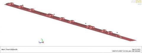
The considered system is represented by a one directional road tunnel model consisting in 800 m length (109 DH, with hydraulic diameter DH=7.3 m), with traffic flow unidirectional and equipped with longitudinal ventilation. The cross section of the tunnel was compliant with ANAS 505(1) standard. The ventilation system used consists of four jet fans, with cross section equal to 0.396 m2, and installed in line, all positioned at 5.60 m above the ground (as reported in the Figure 1). The thrust of jet fans and their spacing were chosen to guarantee that the local velocity value, in optimized system ventilation without fire, tends to the designed velocity value in the proximity of the subsequent inlet jet fan section [2]. The number and diameter of the fans were chosen to achieve a given average air speed in gallery, fixed equal to 3 ms-1, as required PIARC committee [10]. Each fan is provided with cylindrical silencers that, in addition to reducing the sound level, help to keep closed the air flow output.
Figure 1. Traffic distribution used for CFD simulation
3.2 Numerical approach: governing equations
The governing equations of the fluid region for three-dimensional flux are time Averaged mass Navier Stokes in both steady and turbulent states [11]. The Navier Stokes equations are combined with k-$\varepsilon$ realizable model. Transport equations of k-realizable model are reported in Eqs(7) and Eq(8):
$\frac{\partial}{\partial x}(\rho \varepsilon u)+\frac{\partial}{\partial y}(\rho \varepsilon v)+\frac{\partial}{\partial z}(\rho \varepsilon w)=\frac{\partial}{\partial x}\left[\left(\mu+\frac{\mu_{t}}{\sigma_{z}}\right) \frac{\partial \varepsilon}{\partial x}\right]+\frac{\partial}{\partial y}\left[\left(\mu+\frac{\mu_{t}}{\sigma_{z}}\right) \frac{\partial \varepsilon}{\partial y}\right]+$$+\frac{\partial}{\partial z}\left[\left(\mu+\frac{\mu_{t}}{\sigma_{z}}\right) \frac{\partial \varepsilon}{\partial z}\right]+\rho C_{1} S \varepsilon-\rho C_{2} \frac{\varepsilon^{2}}{k+\sqrt{v \varepsilon}}+C_{1 \varepsilon} \frac{\varepsilon}{k} C_{3 \varepsilon} G_{b}$(7)
$\begin{align} & \frac{\partial }{\partial x}\left( \rho ku \right)+\frac{\partial }{\partial y}\left( \rho kv \right)+\frac{\partial }{\partial z}\left( \rho kw \right)=\frac{\partial }{\partial x}\left[ \left( \mu +\frac{{{\mu }_{t}}}{{{\sigma }_{z}}} \right)\frac{\partial k}{\partial x} \right]+\frac{\partial }{\partial y}\left[ \left( \mu +\frac{{{\mu }_{t}}}{{{\sigma }_{z}}} \right)\frac{\partial k}{\partial y} \right]+ \\ & \\ \end{align}$$+\frac{\partial }{\partial z}\left[ \left( \mu +\frac{{{\mu }_{t}}}{{{\sigma }_{z}}} \right)\frac{\partial k}{\partial z} \right]+{{G}_{k}}-{{G}_{b}}-\rho \eta +{{Y}_{M}}$ (8)
The turbulent dynamic viscosity, $\mu$t, is predicted from the knowledge of both the turbulent kinetic energy k, and the turbulent kinetic energy dissipation rate, $\varepsilon$. The transport equations for k and $\varepsilon$ are formulated using the Realizable k-$\varepsilon$ model. They can be derived from Navier-Stokes equations, but the constants in $\varepsilon$ equation are derived using Realizable theory, as suggested in [11].
3.3 Hypotheses and boundary conditions
3.3.1 Hypotheses
In this CFD analysis the following hypotheses are imposed:
-the swirl component due to the air flux passage through the fan wheel is neglected;
-vehicle (car and truck) resistance coefficients (CD) are fixed equal to 1, since vehicles were modeled as blocks in the wind tunnel (when the flow direction is from back to front of them, is almost independent of the type of car, [1]);
-the distance between two subsequent vehicles is equal to 2 m; vehicles traffic is composed of 12% of trucks and of 88% of cars: it is set in two-lines;
-vehicle dimensions are summarized in the Table 1: the car and truck sections area are equal to 2.0 m2 and 7.0 m2 respectively;
-in the traffic jam configuration, the vehicles were modeled as solid blocks (parallelepiped shape);
-average air velocity is equal to 3 ms-1.
Table 1. Vehicle dimensions
|
|
vehicle dimensions /m |
||
|
|
height/m |
length/m |
width/m |
|
car |
1.6 |
4 |
2 |
|
truck |
3 |
12 |
2.2 |
-air properties, considered as an ideal gas, are assumed constant with the temperature and evaluated at the ambient temperature;
-air temperature is assumed equal to 288 K;
-Dp is considered as function of FTP;
-the values of tunnel ceiling and floor roughness are equal to 0.03 m and 0.01 m respectively;
-the value of car and truck roughness is equal to 0.01 m;
-turbulent model: k-e realizable.
3.3.3 Mesh analysis
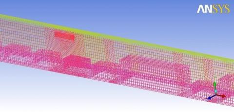
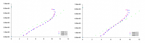
The jet fans was discretized by means hexahedral of 0.2 m height with triangular base of 0.1 m, instead for the tunnel a hexahedral and tetrahedral discretization was used, as shown in Figure 2. In Table 2 the simulations analyzed are summarized. The mesh analysis was carried out in terms of air average velocity in the tunnel at different distances (4 m, 10 m, 20 m, 30 m, 40 m e 50 m) from the jet fan on symmetry plane, as presented in the Figures 3.a-3.f. The 0.4 m mesh size along x-axes represents an acceptable compromise between the accuracy of numerical results and the computational time.
Figure 2. Mesh type
Table 2. Analyzed configurations, with reference to the Figure 2
|
Configuration |
Lateral block |
|
|
hexahedral elementsize/m |
tetrahedral element size/m |
|
|
1 |
0.5 |
0.5 |
|
2 |
0.4 |
0.4 |
|
3 |
0.3 |
0.3 |
The CFD simulation was conducted for different Filling Percentage of the tunnel Traffic (0 to 100% by 10% step); vehicle traffic was composed by 12% of trucks and 88% of cars. The traffic distribution in a random configuration was reported in Figure 1. The authors have investigated the losses due to the presence of vehicles in different traffic conditions: from empty tunnel to 100 % tunnel filled by 10% step (20 cars and 2 trucks). The additional thrust required to balance the losses due to vehicles was evaluated by Eq(9):
DL=LT - LRT(9)
where LT is the thrust required in the case of tunnel with traffic and LRT considers the case of empty tunnel. The Table 3 and the Figure 4 summarize the CFD results and compare them with those provided by semi-empirical formula. The results shows that the semi-empirical formula underestimates the pressure losses with respect to CFD up to 70% of FPT value; the opposite happens for FPT value greater than 70%. The underestimation of the pressure losses is probably due to the fact that semi-empirical formula does not take into account properly the presence of jet fans. In fact, the velocity of the air accelerated by jet fan is greater in proximity of ceiling than in lower zone near the vehicles.
Figure 3. Mesh analysis in terms of average air velocity for different distance values from the jet fan
Table 3. Comparison between CFD and semi-empirical results
|
|
semi-empirical formula |
CFD |
|||
|
FTP/% |
Lvehicles/N |
pressure losses Dpvehicles /Pa |
Pressure drop jet fans Dpfan/Pa |
Thrust jet provided by fans LT/N |
Additional thrust for vehicles Lvehicles/N |
|
0 |
0 |
0 |
1.500 |
2.375 |
0 |
|
10 |
352 |
600 |
2.100 |
3.325 |
950 |
|
20 |
704 |
700 |
2.200 |
3.484 |
1.109 |
|
30 |
1.056 |
900 |
2.400 |
3.801 |
1.426 |
|
40 |
1.408 |
1.200 |
2.700 |
4.276 |
1.901 |
|
50 |
1.760 |
1.300 |
2.800 |
4.434 |
2.059 |
|
60 |
2.112 |
1.500 |
3.000 |
4.751 |
2.376 |
|
70 |
2.464 |
1.600 |
3.100 |
4.909 |
2.534 |
|
80 |
2.816 |
1.700 |
3.200 |
5.068 |
2.693 |
|
90 |
3.168 |
2.000 |
3.500 |
5.543 |
3.168 |
|
100 |
3.520 |
2.100 |
3.600 |
5.701 |
3.326 |
Figure 4. Comparison between losses due to the CFD simulation and semi-empirical formula given by eq. (3) versus FTP%
Furthermore the semi-empirical formula does not take into account the “air ducting” effect due to queuing of vehicles. In particular, the air ducting effect consists in "preferential” channel which is generated above the vehicle, through which the airflow passes without suffering the effects backside of vehicles; this causes mainly friction on the roof of the vehicles than on lateral vehicle surface.
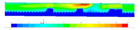
Figure 5 shows tunnel velocity field on plane passing on symmetry section of vehicles; one notes that the velocity of the air accelerated by jet fan in presence of traffic causes the ducting effect. In fact, due to the longitudinal ventilation systems, the velocity of the air is greater in proximity of the ceiling than of the floor.
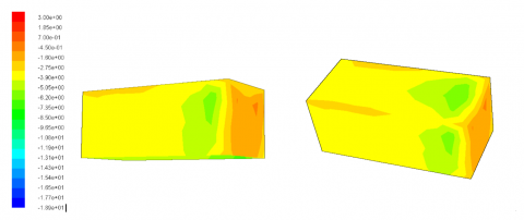
As shown in the Figure 6, the high pressure field occurs on roof of truck and depends also on the relative position between truck and jet fan. The Figures 7 and 8 show the pressure fields on a single car in empty tunnel and in traffic jam conditions. One notes that in the first case the pressure is higher on back and lateral side of vehicle, in the second case the pressure is higher on roof.
Figure 5. Tunnel velocity field for filled traffic configuration
Figure 6. Tunnel pressure field for filled traffic configuration
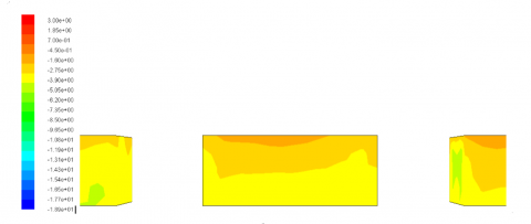
Figure 7. Pressure profile for a single vehicle in empty tunnel configuration: a) lateral view; b) up view
Figure 8. Side view of pressure profile in filled traffic tunnel configuration
The CFD technique has been applied to model several traffic jam conditions fixing the tunnel geometry and the average axial velocity (equal to 3 ms-1). The authors have evaluated the influence of Filling Percentage Traffic (FPT) of the tunnel in presence of longitudinal ventilation system. The simulations have highlighted that the semi-empirical relation based on principle of additively tends to underestimate losses for FPT less than 70%, and overestimate for FPT greater than 70%. The semi-empirical correlation fails for two mainly aspect: i) do not take into account the actual ventilation systems and ii) it does not evaluate properly the ducting effect due to the queuing of vehicles.
|
Afan |
Jet fan cross section, m2 |
|
|
Ai |
Vehicle cross section, m2 |
|
|
At |
Tunnel cross section, m2 |
|
|
Avehicle |
Total vehicle cross section, m2 |
|
|
$C_{1\varepsilon}$, $C_{2\varepsilon}$ |
Model constants, (-) |
|
|
CD |
Vehicle drag coefficient, (-) |
|
|
cp |
Specific heat at constant pressure, J kg-1K-1 |
|
|
f |
Friction coefficient, (-) |
|
|
g |
Gravity acceleration, ms-2 |
|
|
k |
Turbulent kinetic energy, m2 s-2 |
|
|
kg |
Grade correction factor, (-) |
|
|
DH |
Tunnel hydraulic diameter, m |
|
|
Lt |
Tunnel length, m |
|
|
Gb |
Generation of turbulent kinetic energy due to the buoyancy, kg·m-1s-3 |
|
|
Gk nj |
Generation of turbulent kinetic energy due to the mean velocity gradient, kg·m-1s-3 Number of jet fan, (-) |
|
|
Ni |
Amount of a particular vehicle type, (-) |
|
|
Q |
Heat release rate, W |
|
|
T u, v, w |
Temperature, K Air velocity components, m s-1 |
|
|
uv ut |
Tunnel average air velocity, m s-1 Average vehicle velocity, m s-1 |
|
|
x,y,z |
Cartesian coordinates, m |
|
|
Greek symbols |
|
|
|
$\varepsilon$ |
Dissipation rate of turbulent kinetic energy, m2 s-3 |
|
|
$\lambda$ |
Friction factor or Fanning number (Moody’s abacus) |
|
|
$\mu$ |
Dynamic viscosity, Pa s |
|
|
$\mu_t$ |
Dynamic turbulent viscosity, Pa s |
|
|
$\rho$ |
Air density, kg m-3 |
|
|
$\sigma$ |
Turbulent Prandtl Number (-) |
|
|
Subscripts |
|
|
|
i, j, l |
Indexes |
|
|
k $\varepsilon$ |
Turbulent kinetic Energy Dissipation rate of turbulent kinetic energy |
|
[1] Eftekharian E., Abouali O. and Ahmadi G., “A numerical investigation into the performance of two types of jet fans in ventilation of an urban tunnel under traffic jam condition,” Tunnelling and Underground Space Technology, vol. 44, pp. 56–67, 2014.
[2] Betta V., Cascetta F., Musto M. and Rotondo G., “Fluid dynamic performances of traditional and alternative jet fans in tunnel longitudinal ventilation systems,” Tunnelling and Underground Space Technology, vol. 25, pp. 415-422, 2010.
[3] Betta V., Cascetta F., Musto M. and Rotondo G, “Numerical study of the optimization of the pitch angle of an alternative jet fan in a longitudinal tunnel ventilation system,” Tunnelling and Underground Space Technology, vol. 24, pp. 164-172, 2009.
[4] Musto M. and Rotondo G., “Numerical comparison of performance between traditional and alternative jet fans in tiled tunnel in emergency ventilation,” Tunnelling and Underground Space Technology, vol. 42, pp. 52–58, 2014.
[5] Wang F., Wang M. and Wang Q., “Numerical study of effects of deflected angles of jet fans on the normal ventilation in a curved tunnel,” Tunnelling and Underground Space Technology, vol. 31, pp. 80–85, 2012.
[6] Wang F., Wang M. and HeSDeng Y., “Computational study of effects of traffic force on the ventilation in high way curved tunnels,” Tunnelling and Underground Space Technology, vol. 26, pp. 481–489, 2011.
[7] Wang F., Wang M., Wang Q. and Zhao D., “An improved model of traffic force based on CFD in a curved tunnel,” Tunnelling and Underground Space Technology, vol. 4, pp. 120-126, 2014.
[8] Eftekharian E., Abouali O. and Ahmadi G., “An improved correlation for pressure drop in a tunnel under traffic jam using CFD,” Journal of Wind Eng. Ind. Aerodyn., vol. 143, pp. 34–41, 2015.
[9] The 9th International Conference on Aerodynamics and Ventilation of Vehicle tunnels. 6-8 October 1997, Aosta Italy.
[10] World Road Association, Road Tunnels, 2012. Vehicle emissions and air demand for ventilation. PIARC Committee on Road Tunnels Operation (C4).
[11] Fluent, User’s Guide, 2005 Fluent Inc.